Quarto with R

Abstrave quarto theme

Roy Francis

05-Sep-2026

Introduction

This Quarto Reveal.js presentation demonstrates executable R code, R output, and R-backed interactive content.

Render a presentation from R with quarto::quarto_render().

quarto::quarto_render("example.qmd")

Code

Inline R code is evaluated within text content. This text `r Sys.Date()` produces this: 2026-09-05.

R code is executed inside R code chunks.

```{r}
Sys.Date()
```

Code chunks display their code and output by default.

Sys.Date()

[1] "2026-09-05"

Hide code or output

Chunk options can control the display of source and results.

Hide source code:

```{r}
#| echo: false
data(iris)
```

Sepal.Length	Sepal.Width
5.1	3.5
4.9	3.0
4.7	3.2

Hide output:

```{r}
#| results: "hide"
Sys.Date()
```

Sys.Date()

Code folding

Source code can be folded while keeping output visible.

```{r}
#| code-fold: true
Sys.Date()
```

Code

Sys.Date()

[1] "2026-09-05"

The mcanouil/collapse-output extension can be used to fold output.

Sys.Date()

Code Output

[1] "2026-09-05"

Code sizing

Source code

Sys.Date()

[1] "2026-09-05"

Sys.Date()

[1] "2026-09-05"

Source and output

Sys.Date()

[1] "2026-09-05"

Sys.Date()

[1] "2026-09-05"

Code highlighting

```{r}
#| code-line-numbers: "2-3"
iris |>
  head() |>
  knitr::kable()
```

iris |>
  head() |>
  knitr::kable()

Sepal.Length	Sepal.Width	Petal.Length	Petal.Width	Species
5.1	3.5	1.4	0.2	setosa
4.9	3.0	1.4	0.2	setosa
4.7	3.2	1.3	0.2	setosa
4.6	3.1	1.5	0.2	setosa
5.0	3.6	1.4	0.2	setosa
5.4	3.9	1.7	0.4	setosa

Images with knitr

R chunks can use out-width to control image dimensions.

```{r}
#| echo: false
#| out-width: "100px"
knitr::include_graphics("assets/image.webp")
```

Tables • kable

The most simple table using kable from R package knitr.

knitr::kable(head(iris), "html")

Sepal.Length	Sepal.Width	Petal.Length	Petal.Width	Species
5.1	3.5	1.4	0.2	setosa
4.9	3.0	1.4	0.2	setosa
4.7	3.2	1.3	0.2	setosa
4.6	3.1	1.5	0.2	setosa
5.0	3.6	1.4	0.2	setosa
5.4	3.9	1.7	0.4	setosa

Tables • gt

Tables using the gt package. Grammar of tables with extensive customization options.

library(gt)
iris |>
  group_by(Species) |>
  slice(1:2) |>
  gt() |>
  cols_label(Sepal.Length = "Sepal Length", Sepal.Width = "Sepal Width")

Sepal Length	Sepal Width	Petal.Length	Petal.Width
setosa
5.1	3.5	1.4	0.2
4.9	3.0	1.4	0.2
versicolor
7.0	3.2	4.7	1.4
6.4	3.2	4.5	1.5
virginica
6.3	3.3	6.0	2.5
5.8	2.7	5.1	1.9

Tables • kableExtra

More advanced table using kableExtra and formattable.

 iris[c(1:2,51:52,105:106),] |>
  mutate(Sepal.Length=color_bar("lightsteelblue")(Sepal.Length)) |>
  mutate(Sepal.Width=color_tile("white","orange")(Sepal.Width)) |>
  mutate(Species=cell_spec(Species,"html",color="white",bold=T,
    background=c("#8dd3c7","#fb8072","#bebada")[factor(Species)])) |>
  kable("html",escape=F) |>
  kable_styling(bootstrap_options=c("striped","hover","responsive"),full_width=F) |>
  column_spec(5,width="3cm")

	Sepal.Length	Sepal.Width	Petal.Length	Petal.Width	Species
1	5.1	3.5	1.4	0.2	setosa
2	4.9	3.0	1.4	0.2	setosa
51	7.0	3.2	4.7	1.4	versicolor
52	6.4	3.2	4.5	1.5	versicolor
105	6.5	3.0	5.8	2.2	virginica
106	7.6	3.0	6.6	2.1	virginica

Interactive tables • DT

Interactive table using R package DT.

library(DT)
DT::datatable(iris[1:20, ], options = list(pageLength = 7))

Interactive tables • reactable

Interactive tables with reactable.

library(reactable)
reactable(iris[sample(1:150, 6), ], striped = TRUE, highlight = TRUE, filterable = TRUE)

Static plots • base R

par(mar = c(5, 5, 0, 0))
plot(
  x = iris$Sepal.Length, y = iris$Sepal.Width,
  col = c("coral", "steelblue", "forestgreen")[iris$Species],
  xlab = "Sepal Length", ylab = "Sepal Width", pch = 19
)
legend("bottomright", legend = levels(iris$Species), col = c("coral", "steelblue", "forestgreen"), pch = 19)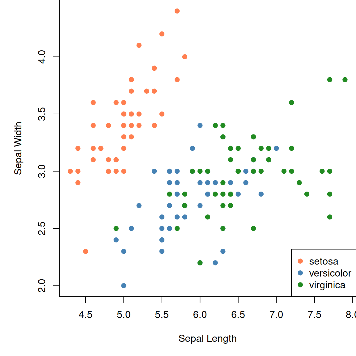

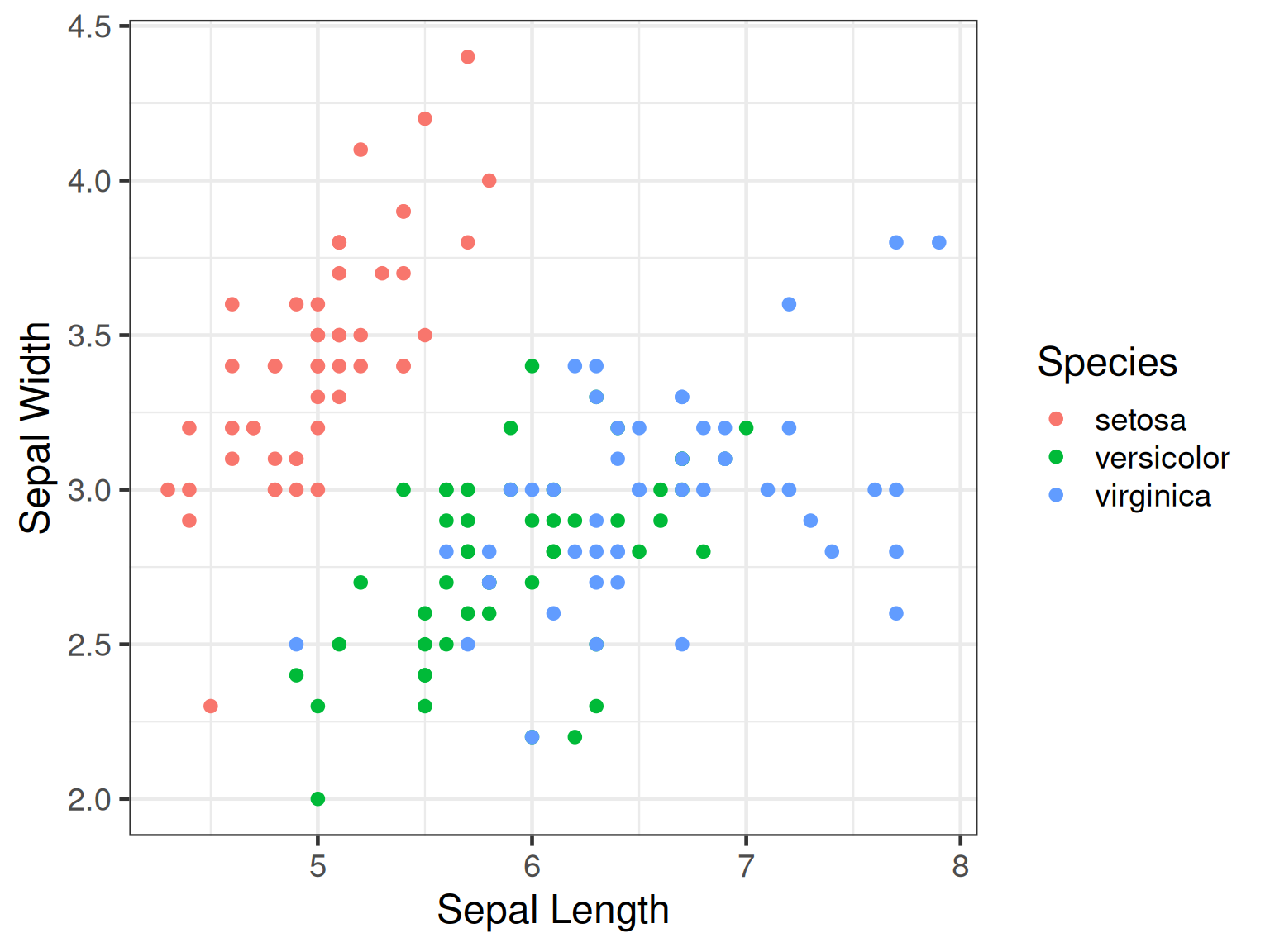
Static plots • ggplot2

Plotting using ggplot2.

iris |>
  ggplot(aes(x = Sepal.Length, y = Sepal.Width, colour = Species)) +
  geom_point(size = 2) +
  labs(x = "Sepal Length", y = "Sepal Width") +
  theme_bw(base_size = 18)

Interactive time series • `dygraphs`

R package dygraphs provides R bindings for javascript library dygraphs for time series data.

library(dygraphs)
lungDeaths <- cbind(ldeaths, mdeaths, fdeaths)
dygraph(lungDeaths,main="Deaths from Lung Disease (UK)") |>
  dyOptions(colors=c("#66C2A5","#FC8D62","#8DA0CB"))

Interactive plots • highcharter

R package highcharter is a wrapper around javascript library highcharts.

library(highcharter)
h <- iris |>
  hchart("scatter", hcaes(x = "Sepal.Length", y = "Sepal.Width", group = "Species")) |>
  hc_xAxis(title = list(text = "Sepal Length"), crosshair = TRUE) |>
  hc_yAxis(title = list(text = "Sepal Width"), crosshair = TRUE) |>
  hc_chart(zoomType = "xy") |>
  hc_size(height = 300, width = 500)
htmltools::tagList(h)

Interactive plots • plotly

R package plotly provides R binding around javascript plotting library plotly.

library(plotly)
iris |>
  plot_ly(x = ~Sepal.Length, y = ~Sepal.Width, color = ~Species, width = 550, height = 400) |>
  add_markers()

Interactive plots • plotly • ggplotly

plotly has a function called ggplotly which converts a static ggplot2 object into an interactive plot.

library(plotly)
p <- ggplot(iris, aes(x = Sepal.Length, y = Sepal.Width, colour = Species)) +
  geom_point() +
  theme_bw(base_size = 12)

plotly::ggplotly(p, width = 460, height = 360)

Interactive plots • ggiraph

R package ggiraph converts a static ggplot2 object into an interactive plot.

library(ggiraph)
p <- ggplot(iris,aes(x=Sepal.Length,y=Petal.Length,colour=Species))+
      geom_point_interactive(aes(tooltip=paste0("<b>Petal Length:</b> ",Petal.Length,"\n<b>Sepal Length: </b>",Sepal.Length,"\n<b>Species: </b>",Species)),size=1)+
  theme_bw()
tooltip_css <- "background-color:#f8f9f9;padding:10px;border-style:solid;border-width:2px;border-color:#125687;border-radius:5px;"
girafe(code=print(p), height_svg=1.5, width_svg=3.5,
  options=list(opts_hover(css="cursor:pointer;stroke:black;fill-opacity:0.3"), opts_zoom(max=5),
    opts_tooltip(css=tooltip_css,opacity=0.9), opts_sizing(width=0.6)))

Network graph • networkD3

R package networkD3 allows the use of interactive network graphs from the D3.js javascript library.

library(networkD3)
data(MisLinks,MisNodes)
forceNetwork(Links=MisLinks,Nodes=MisNodes,Source="source",
             Target="target",Value="value",NodeID="name",
             Group="group",opacity=0.4,
             height=300,width=500)

Interactive maps • Leaflet

R package leaflet provides R bindings for javascript mapping library; leafletjs.

library(leaflet)
leaflet(height = 300, width = 800) |>
  addTiles(
    urlTemplate = 'https://{s}.tile.openstreetmap.org/{z}/{x}/{y}.png'
  ) |>
  #addProviderTiles(providers$Esri.NatGeoWorldMap) |>
  addMarkers(lat = 57.639327, lng = 18.288534, popup = "RaukR") |>
  setView(lat = 57.639327, lng = 18.288534, zoom = 15)

Linking plots • crosstalk

R package crosstalk allows crosstalk enabled plotting libraries to be linked. Through the shared ‘key’ variable, data points can be manipulated simultaneously on two independent plots.

library(crosstalk)
shared_quakes <- SharedData$new(quakes[sample(nrow(quakes), 100),])
lf <- leaflet(shared_quakes,height=300) |>
        addTiles(urlTemplate='http://{s}.tile.openstreetmap.org/{z}/{x}/{y}.png') |>
        addMarkers()
py <- plot_ly(shared_quakes,x=~depth,y=~mag,size=~stations,height=300) |> add_markers()
div(div(lf,style="float:left;width:49%"),div(py,style="float:right;width:49%"))

ObservableJS

Quarto supports ObservableJS for interactive visualisations in the browser.

Pass data from R to OJS

irism <- iris
colnames(irism) <- gsub("[.]","_",tolower(colnames(irism)))
ojs_define(ojsd = irism)

ojsdata = transpose(ojsd)

Display as a table

viewof filtered_table = Inputs.table(ojsdata)

ObservableJS

Define inputs

viewof x = Inputs.select(Object.keys(ojsdata[0]), {
  value: "sepal_length", multiple: false, label: "X axis"
  })

viewof y = Inputs.select(Object.keys(ojsdata[0]), {
  value: "sepal_width", multiple: false, label: "Y axis"
  })

Display plot

Plot.plot({
  marks: [
    Plot.dot(ojsdata, {
      x: x, y: y, fill: "species",
      title: (d) => `${d.species} \n Petal length: ${d.petal_length} \n Sepal length: ${d.sepal_length}`
    })
  ], grid: true
})

ObservableJS in quarto documentation.

Session

If content overflows a slide vertically, add the .scrollable class.

::: {.scrollable}
<contents>
:::

R version 4.6.1 (2026-06-24)
Platform: x86_64-pc-linux-gnu
Running under: Ubuntu 24.04.4 LTS

Matrix products: default
BLAS:   /usr/lib/x86_64-linux-gnu/openblas-pthread/libblas.so.3 
LAPACK: /usr/lib/x86_64-linux-gnu/openblas-pthread/libopenblasp-r0.3.26.so;  LAPACK version 3.12.0

locale:
 [1] LC_CTYPE=C.UTF-8       LC_NUMERIC=C           LC_TIME=C.UTF-8       
 [4] LC_COLLATE=C.UTF-8     LC_MONETARY=C.UTF-8    LC_MESSAGES=C.UTF-8   
 [7] LC_PAPER=C.UTF-8       LC_NAME=C              LC_ADDRESS=C          
[10] LC_TELEPHONE=C         LC_MEASUREMENT=C.UTF-8 LC_IDENTIFICATION=C   

time zone: UTC
tzcode source: system (glibc)

attached base packages:
[1] stats     graphics  grDevices utils     datasets  methods   base     

other attached packages:
 [1] dygraphs_1.1.1.6  gt_1.3.0          crosstalk_1.2.2   leaflet_2.2.3    
 [5] networkD3_0.4.1   ggiraph_0.9.6     plotly_4.12.1     highcharter_0.9.5
 [9] htmltools_0.5.9   ggplot2_4.0.3     reactable_0.4.5   DT_0.34.0        
[13] formattable_0.2.1 kableExtra_1.4.1  stringr_1.6.0     tidyr_1.3.2      
[17] dplyr_1.2.1      

loaded via a namespace (and not attached):
 [1] tidyselect_1.2.1        viridisLite_0.4.3       farver_2.1.2           
 [4] S7_0.2.2                fastmap_1.2.0           fontquiver_0.2.1       
 [7] digest_0.6.39           timechange_0.4.0        lifecycle_1.0.5        
[10] magrittr_2.0.5          compiler_4.6.1          rlang_1.3.0            
[13] sass_0.4.10             tools_4.6.1             igraph_2.3.3           
[16] yaml_2.3.12             data.table_1.18.6.1     knitr_1.51             
[19] labeling_0.4.3          htmlwidgets_1.6.4       curl_8.0.0             
[22] xml2_1.6.0              TTR_0.24.4              RColorBrewer_1.1-3     
[25] withr_3.0.3             purrr_1.2.2             grid_4.6.1             
[28] gdtools_0.5.1           xts_0.14.2              data.tree_1.2.0        
[31] scales_1.4.0            MASS_7.3-65             cli_3.6.6              
[34] rmarkdown_2.32          generics_0.1.4          otel_0.2.0             
[37] rlist_0.4.6.2           rstudioapi_0.19.0       httr_1.4.9             
[40] cachem_1.1.0            assertthat_0.2.1        vctrs_0.7.3            
[43] jsonlite_2.0.0          fontBitstreamVera_0.1.1 systemfonts_1.3.2      
[46] jquerylib_0.1.4         quantmod_0.4.29         glue_1.8.1             
[49] reactR_0.6.1            lubridate_1.9.5         stringi_1.8.9          
[52] gtable_0.3.6            tibble_3.3.1            pillar_1.11.1          
[55] R6_2.6.1                textshaping_1.0.5       evaluate_1.0.5         
[58] lattice_0.22-9          backports_1.5.1         broom_1.0.13           
[61] fontLiberation_0.1.0    bslib_0.12.0            Rcpp_1.1.2             
[64] svglite_2.2.2           xfun_0.60               fs_2.1.0               
[67] zoo_1.9-0               pkgconfig_2.0.3

Thank you!
Questions?

2026 • Specky

Quarto with R

Introduction

Code

Hide code or output

Code folding

Code sizing

Code highlighting

Images with knitr

Tables • kable

Tables • gt

Tables • kableExtra

Interactive tables • DT

Interactive tables • reactable

Static plots • base R

Static plots • ggplot2

Interactive time series • dygraphs

Interactive plots • highcharter

Interactive plots • plotly

Interactive plots • plotly • ggplotly

Interactive plots • ggiraph

Network graph • networkD3

Interactive maps • Leaflet

Linking plots • crosstalk

ObservableJS

ObservableJS

Session

Interactive time series • `dygraphs`