Quarto demo with R

Abstrave quarto theme

Roy Francis

25-May-2025

Introduction

This is a Quarto revealjs presentation with Abstrave theme. This demo showcases the usage and capabilities of this system. Revealjs in Quarto is documented here.

Getting started

In RStudio, File > New File > Quarto Presentation
Add YAML matter to the top if not already there.

---
title: "This is a title"
format:
  revealjs
---

Click the Render button for a rendered preview.
Or use quarto::quarto_render() in R:

quarto::quarto_render("slide.qmd")

Or use quarto render in the terminal:

quarto render slide.qmd

Slides

Slide separators

Slides are separated by ##. Incremental content on is separated by . . . like below.

Hide or not count a slide:

## Slide Title {visibility="hidden"}
## Slide Title {visibility="uncounted"}

. . .

Slide notes

Any content inside class .notes on a slide are notes. This is only visible in presenter mode (by pressing s).

. . .

Keyboard shortcuts

Press ? for help.

Layout

The slide content can be organized into columns which can be nested if needed.

:::{.columns}
:::{.column width="50%"}
<div style="background-color:#fdebd0">Left content</div>
:::

:::{.column width="50%"}
<div style="background-color:#eaf2f8">Right content</div>

:::{.column width="60%"}
<div style="background-color:#d0ece7">Inner left</div>
:::
:::{.column width="40%"}
<div style="background-color:#f2d7d5">Inner right</div>
:::

:::
:::

Left content

Right content

Inner left

Inner right

Layout • Vertical align • Top

::: {.v-top}
::: {}
- Top aligned
- content
:::
:::

Top aligned
content

Layout • Vertical align • Center

::: {.v-center}
::: {}
- Center aligned
- content
:::
:::

Center aligned
content

Layout • Vertical align • Bottom

::: {.v-bottom}
::: {}
- Bottom aligned
- content
:::
:::

Bottom aligned
content

Content for Tab A

Content for Tab B

Text Formatting

Rendering of normal text, numbers and symbols.

ABCDEFGHIJKLMNOPQRSTUYWXYZÅÄÖ

abcdefghijklmnopqrstuvwxyzåäö

0123456789

!“#%&/()$@*^~<>-:;,_±|?+=

!"#%&/\()$@*^~<>-:;,_±|?+=

Text formatting

Headings can be defined as shown below.

## Level 2 heading  
### Level 3 heading  
#### Level 4 heading  
##### Level 5 heading  
###### Level 6 heading

Level 3 heading

Level 4 heading

Level 5 heading

Level 6 heading

Level 1 usage is not recommended. Use level 2 for slide titles. Use level 3 and below for other titles.

Text scaling classes

[Largest text]{.largest}
[Larger text]{.larger}
[Large text]{.large}
Normal text.  
[Small text]{.small}
[Smaller text]{.smaller}
[Smallest text]{.smallest}

Largest text
Larger text
Large text
Normal text
Small text
Smaller text
Smallest text

Text Formatting

Horizontal alignment of text can be adjusted as shown below.

[Left aligned text]{.left}
[Center aligned text]{.center}
[Right aligned text]{.right}

Left aligned text
Center aligned text
Right aligned text

::: {.blockquote}
This line is quoted
:::

This line is quoted

A horizontal line can be created using ---

This is **Bold text** This is Bold text

This is *Italic text* This is Italic text

~~Strikethrough~~ text ~~Strikethrough~~ text

This is subscript H~2~O H₂O

This is superscript 2^10^ 2¹⁰

This is a [badge]{.badge .badge-primary}
This is a badge

This is a [badge]{.badge .badge-secondary}
This is a badge

This is a [link](r-project.org) This is a link

Text formatting

Fit text to full width.

::: {.r-fit-text}
Attention
:::

Attention

Text formatting

In reports, .aside pushes content into the margin while in revealjs, it is pushed to the bottom.

::: {.aside}
Content inside aside.
:::

Lists

Unordered List

- Bullet 1
- Bullet 2
  - Sub-bullet 2.1

Bullet 1
Bullet 2
- Sub-bullet 2.1

Incremental List

:::{.incremental}
1. Incremental Bullet 1
2. Incremental Bullet 2
3. Incremental Bullet 3
:::

Incremental Bullet 1
Incremental Bullet 2
Incremental Bullet 3

For more options, see here.

Custom CSS styling

You can style text using any custom CSS
This is a block level element

::: {style="color: red"}
This paragraph is red.
:::

This paragraph is red.

This is a span. ie; A word or one line.

[This text is blue]{style="color: blue"}

This text is blue

Callouts

::: {.callout-note}
This is a callout.
:::

::: {.callout-warning}
This is a callout.
:::

::: {.callout-important}
This is a callout.
:::

::: {.callout-tip}
This is a callout.
:::

::: {.callout-caution}
This is a callout.
:::

Note

This is a callout.

Warning

This is a callout.

Important

This is a callout.

Tip

This is a callout.

Caution

This is a callout.

Callouts

Variants of callout

::: {.callout-note icon=false}
Icon is disabled
:::

::: {.callout-note appearance="simple"}
Appearance is simple
:::

::: {.callout-note appearance="minimal"}
Appearance is minimal
:::

::: {.callout-note appearance="simple"}
## Custom title
Simple appearance and a custom title
:::

::: {.callout-note appearance="minimal"}
## Custom title
Minimal appearance and a custom title
:::

Note

Icon is disabled

Appearance is simple

Appearance is minimal

Custom title

Simple appearance and a custom title

Custom title

Minimal appearance and a custom title

Callouts

::: {.callout-note}

This contains code

## Callout with code

```
Sys.Date()
```

:::

Callout with code

This contains code

Sys.Date()

Code formatting

Inline code

Code can be defined inline where `this` looks like this.
R code can be executed inline `r Sys.Date()` producing 2025-05-25.

== != && ++ |> <> <- <= <~ /= |=> ->>

Code formatting

Code chunks

Code can also be defined inside chunks.

```
This is code
```

This is code

R code is executed inside code blocks like this

```{r}
Sys.Date()
```

which shows the code and output.

Sys.Date()

[1] "2025-05-25"

The code and results can be hidden by

```{r}
#| echo: false
#| results: hide
data(iris)
```

data(iris)
head(iris[1:3,1:2])

Sepal.Length	Sepal.Width
5.1	3.5
4.9	3.0
4.7	3.2

These are called chunk attributes. For more options, see here and complete list here.

Code highlighting

```{r}
#| eval: false
#| echo: true
#| code-line-numbers: "2-3"

iris %>%
  ggplot(aes(x=Sepal.Length,y=Sepal.Width,col=Species))+
  geom_point(size=2)+
  labs(x="Sepal Length",y="Sepal Width")+
  theme_report()
```

iris %>%
  ggplot(aes(x=Sepal.Length,y=Sepal.Width,col=Species))+
  geom_point(size=2)+
  labs(x="Sepal Length",y="Sepal Width")+
  theme_report()

```{r}
#| eval: false
#| echo: true
#| code-line-numbers: "2|3|5"

iris %>%
  ggplot(aes(x=Sepal.Length,y=Sepal.Width,col=Species))+
  geom_point(size=2)+
  labs(x="Sepal Length",y="Sepal Width")+
  theme_report()
```

iris %>%
  ggplot(aes(x=Sepal.Length,y=Sepal.Width,col=Species))+
  geom_point(size=2)+
  labs(x="Sepal Length",y="Sepal Width")+
  theme_report()

For more code highlighting documentation, see here.

Images • Markdown

Using Markdown

Using regular markdown.

![](assets/image.webp)

The dimensions are based on image and/or fill up the entire width.

Control image dimensions.

![](assets/image.webp){width=50%}
![](assets/image.webp){width=20%}

For more image documentation, see here.

Images • Markdown • Layout

Figure layout

::: {layout-ncol=3}
![Caption for figure 1](assets/image.webp){#fig-layout-1}

![Caption for figure 2](assets/image.webp){#fig-layout-2}

![Caption for figure 3](assets/image.webp){#fig-layout-3}
:::

Images • Markdown • Layout

Absolute positioning

![](assets/image.webp){.absolute top=250 left=0 height="450"}
![](assets/image.webp){.absolute top=200 right=50 height="250"}
![](assets/image.webp){.absolute bottom=0 right=200 height="200"}

Images • HTML

Using Raw HTML

This image is 30% size. <img src="assets/image.webp" style="width:30%;"/>

Images • R

Using R

R chunks in RMarkdown can be used to control image display size using the argument out.width.

This image is displayed at a size of 200 pixels.

```{r}
#| out-width: "200px"
knitr::include_graphics("assets/image.webp")
```

Stacking

Stack images and display incrementally

::: {.r-stack}
::: {.fragment}

![](assets/image.webp){style="transform:rotate(-5deg);border:beige 40px solid;"}

:::
::: {.fragment}

![](assets/image.webp){style="transform:rotate(5deg);border:beige 40px solid;"}

:::
:::

Stretching

Stretch images to use up remaining space.

![](assets/image.webp){.stretch}

Math expressions

Some examples of rendering equations.

$e^{i\pi} + 1 = 0$

$$\frac{E \times X^2 \prod I}{2+7} = 432$$

$$\sum_{i=1}^n X_i$$

$$\int_0^{2\pi} \sin x~dx$$

$e^{i\pi} + 1 = 0$ \[\frac{E \times X^2 \prod I}{2+7} = 432\] \[\sum_{i=1}^n X_i\] \[\int_0^{2\pi} \sin x~dx\]

Math expressions

Some examples of rendering equations.

$\left( \sum_{i=1}^{n}{i} \right)^2 = \left( \frac{n(n-1)}{2}\right)^2 = \frac{n^2(n-1)^2}{4}$

$\begin{eqnarray} X & \sim & \mathrm{N}(0,1)\\ Y & \sim & \chi^2_{n-p}\\ R & \equiv & X/Y \sim t_{n-p} \end{eqnarray}$

$\begin{eqnarray} P(|X-\mu| > k) & = & P(|X-\mu|^2 > k^2)\\ & \leq & \frac{\mathbb{E}\left[|X-\mu|^2\right]}{k^2}\\ & \leq & \frac{\mathrm{Var}[X]}{k^2} \end{eqnarray}$

$\left( \sum_{i=1}^{n}{i} \right)^2 = \left( \frac{n(n-1)}{2}\right)^2 = \frac{n^2(n-1)^2}{4}$

$\begin{eqnarray} X & \sim & \mathrm{N}(0,1)\\ Y & \sim & \chi^2_{n-p}\\ R & \equiv & X/Y \sim t_{n-p} \end{eqnarray}$

$\begin{eqnarray} P(|X-\mu| > k) & = & P(|X-\mu|^2 > k^2)\\ & \leq & \frac{\mathbb{E}\left[|X-\mu|^2\right]}{k^2}\\ & \leq & \frac{\mathrm{Var}[X]}{k^2} \end{eqnarray}$

Tables • `kable`

The most simple table using kable from R package knitr.

knitr::kable(head(iris),'html')

Sepal.Length	Sepal.Width	Petal.Length	Petal.Width	Species
5.1	3.5	1.4	0.2	setosa
4.9	3.0	1.4	0.2	setosa
4.7	3.2	1.3	0.2	setosa
4.6	3.1	1.5	0.2	setosa
5.0	3.6	1.4	0.2	setosa
5.4	3.9	1.7	0.4	setosa

Tables • gt

Tables using the gt package. Grammar of tables with extensive customization options.

library(gt)

iris %>%
    group_by(Species) %>%
    slice(1:2) %>%
    gt() %>%
    cols_label(
      Sepal.Length = "Sepal Length", Sepal.Width = "Sepal Width",
      Petal.Length = "Petal Length", Petal.Width = "Petal Width"
    ) %>%
    tab_source_note(
        source_note = md("Source: Iris data. Anderson, 1936; Fisher, 1936)")
    )

Sepal Length	Sepal Width	Petal Length	Petal Width
setosa
5.1	3.5	1.4	0.2
4.9	3.0	1.4	0.2
versicolor
7.0	3.2	4.7	1.4
6.4	3.2	4.5	1.5
virginica
6.3	3.3	6.0	2.5
5.8	2.7	5.1	1.9
Source: Iris data. Anderson, 1936; Fisher, 1936)

Tables • `kableExtra`

More advanced table using kableExtra and formattable.

 iris[c(1:2,51:52,105:106),] %>%
  mutate(Sepal.Length=color_bar("lightsteelblue")(Sepal.Length)) %>%
  mutate(Sepal.Width=color_tile("white","orange")(Sepal.Width)) %>%
  mutate(Species=cell_spec(Species,"html",color="white",bold=T,
    background=c("#8dd3c7","#fb8072","#bebada")[factor(.$Species)])) %>%
  kable("html",escape=F) %>%
  kable_styling(bootstrap_options=c("striped","hover","responsive"),full_width=F) %>%
  column_spec(5,width="3cm")

	Sepal.Length	Sepal.Width	Petal.Length	Petal.Width	Species
1	5.1	3.5	1.4	0.2	setosa
2	4.9	3.0	1.4	0.2	setosa
51	7.0	3.2	4.7	1.4	versicolor
52	6.4	3.2	4.5	1.5	versicolor
105	6.5	3.0	5.8	2.2	virginica
106	7.6	3.0	6.6	2.1	virginica

Tables • Interactive • `DT`

Interactive table using R package DT.

library(DT)
DT::datatable(iris[1:20,],options=list(pageLength=7))

Tables • Interactive • `reactable`

Interactive tables with reactable.

library(reactable)

reactable(iris[sample(1:150,6),],
  striped = TRUE, highlight = TRUE, filterable = TRUE
)

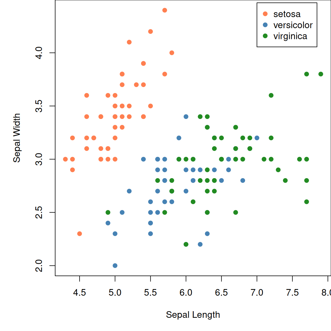
Static plots • Base Plot

Plots using base R.

{par(mar=c(5,5,0,0))
  plot(x=iris$Sepal.Length,y=iris$Sepal.Width,
      col=c("coral","steelblue","forestgreen")[iris$Species],
      xlab="Sepal Length",ylab="Sepal Width",pch=19)
  legend(x=7,y=4.47,legend=c("setosa","versicolor","virginica"),
       col=c("coral","steelblue","forestgreen"),pch=19)}

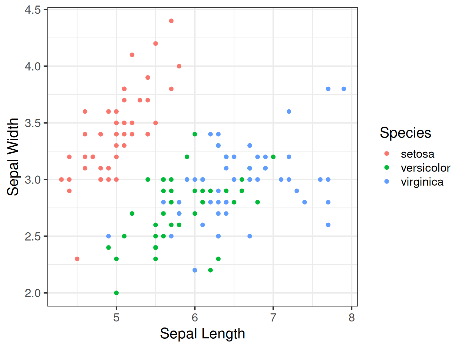
Static plots • `ggplot2`

Plotting using ggplot2.

iris %>%
  ggplot(aes(x=Sepal.Length,y=Sepal.Width,col=Species))+
  geom_point(size=2)+
  labs(x="Sepal Length",y="Sepal Width")+
  theme_bw(base_size=18)

Interactive plots • `highcharter`

R package highcharter is a wrapper around javascript library highcharts.

library(highcharter)
h <- iris %>%
  hchart("scatter",hcaes(x="Sepal.Length",y="Sepal.Width",group="Species")) %>%
  hc_xAxis(title=list(text="Sepal Length"),crosshair=TRUE) %>%
  hc_yAxis(title=list(text="Sepal Width"),crosshair=TRUE) %>%
  hc_chart(zoomType="xy",inverted=FALSE) %>%
  hc_legend(verticalAlign="top",align="right") %>% hc_size(height=300,width=500)
htmltools::tagList(list(h))

Interactive plots • `plotly`

R package plotly provides R binding around javascript plotting library plotly.

library(plotly)
p <- iris %>%
  plot_ly(x=~Sepal.Length,y=~Sepal.Width,color=~Species,width=550,height=400) %>%
  add_markers()
p

Interactive plots • `ggplotly`

plotly also has a function called ggplotly which converts a static ggplot2 object into an interactive plot.

library(plotly)
p <- ggplot(iris,aes(x=Sepal.Length,y=Sepal.Width,col=Species))+
  geom_point()+
  labs(x="Sepal Length",y="Sepal Width")+
  theme_bw(base_size=12)

plotly::ggplotly(p,width=460,height=360)

Interactive plots • `ggiraph`

R package ggiraph converts a static ggplot2 object into an interactive plot.

library(ggiraph)
p <- ggplot(iris,aes(x=Sepal.Length,y=Petal.Length,colour=Species))+
      geom_point_interactive(aes(tooltip=paste0("<b>Petal Length:</b> ",Petal.Length,"\n<b>Sepal Length: </b>",Sepal.Length,"\n<b>Species: </b>",Species)),size=2)+
  theme_bw()
tooltip_css <- "background-color:#f8f9f9;padding:10px;border-style:solid;border-width:2px;border-color:#125687;border-radius:5px;"
girafe(code=print(p), height_svg=2, width_svg=4,
  options=list(
    opts_hover(css="cursor:pointer;stroke:black;fill-opacity:0.3"),
    opts_zoom(max=5),
    opts_tooltip(css=tooltip_css,opacity=0.9),
    opts_sizing(width=0.6)
  )
)

Interactive time series • `dygraphs`

R package dygraphs provides R bindings for javascript library dygraphs for time series data.

library(dygraphs)
lungDeaths <- cbind(ldeaths, mdeaths, fdeaths)
dygraph(lungDeaths,main="Deaths from Lung Disease (UK)") %>%
  dyOptions(colors=c("#66C2A5","#FC8D62","#8DA0CB"))

Network graph

R package networkD3 allows the use of interactive network graphs from the D3.js javascript library.

library(networkD3)
data(MisLinks,MisNodes)
forceNetwork(Links=MisLinks,Nodes=MisNodes,Source="source",
             Target="target",Value="value",NodeID="name",
             Group="group",opacity=0.4,
             height=300,width=500)

Interactive maps • `leaflet`

R package leaflet provides R bindings for javascript mapping library; leafletjs.

library(leaflet)
leaflet(height=300,width=800) %>%
  addTiles(urlTemplate='http://{s}.tile.openstreetmap.org/{z}/{x}/{y}.png') %>%
  #addProviderTiles(providers$Esri.NatGeoWorldMap) %>%
  addMarkers(lat=57.639327,lng=18.288534,popup="RaukR") %>%
  setView(lat=57.639327,lng=18.288534,zoom=15)

Linking Plots • `crosstalk`

R package crosstalk allows crosstalk enabled plotting libraries to be linked. Through the shared ‘key’ variable, data points can be manipulated simultaneously on two independent plots.

library(crosstalk)
shared_quakes <- SharedData$new(quakes[sample(nrow(quakes), 100),])
lf <- leaflet(shared_quakes,height=300) %>%
        addTiles(urlTemplate='http://{s}.tile.openstreetmap.org/{z}/{x}/{y}.png') %>%
        addMarkers()
py <- plot_ly(shared_quakes,x=~depth,y=~mag,size=~stations,height=300) %>%
        add_markers()
div(div(lf,style="float:left;width:49%"),div(py,style="float:right;width:49%"))

ObservableJS

Quarto supports ObservableJS for interactive visualisations in the browser.

Pass data from R to OJS

irism <- iris
colnames(irism) <- gsub("[.]","_",tolower(colnames(irism)))
ojs_define(ojsd = irism)

ojsdata = transpose(ojsd)

Display as a table

viewof filtered_table = Inputs.table(ojsdata)

ObservableJS

Define inputs

viewof x = Inputs.select(Object.keys(ojsdata[0]), {
  value: "sepal_length", multiple: false, label: "X axis"
  })

viewof y = Inputs.select(Object.keys(ojsdata[0]), {
  value: "sepal_width", multiple: false, label: "Y axis"
  })

Display plot

Plot.plot({
  marks: [
    Plot.dot(ojsdata, {
      x: x, y: y, fill: "species",
      title: (d) => `${d.species} \n Petal length: ${d.petal_length} \n Sepal length: ${d.sepal_length}`
    })
  ], grid: true
})

ObservableJS in quarto documentation.

Diagrams

```{mermaid}
flowchart LR
  A[Hard edge] --> B(Round edge)
  B --> C{Decision}
  C --> D[Result one]
  C --> E[Result two]
```

flowchart LR
  A[Hard edge] --> B(Round edge)
  B --> C{Decision}
  C --> D[Result one]
  C --> E[Result two]

Colourful

This slide has a colourful background

##  Colourful {background-color="#ABEBC6"}

Big Image

This slide has a background image

##  Big Image {background-image="assets/image.webp"}

General tips

Replace assets/cover.webp to change cover slide picture
Replace assets/end.webp to change end slide picture
Add custom css under YAML css: "styles.css"
If content overflows the slide in vertical direction, add class .scrollable

                                              sysname 
                                              "Linux" 
                                              release 
                                  "6.11.0-1014-azure" 
                                              version 
"#14~24.04.1-Ubuntu SMP Thu Apr 24 17:41:03 UTC 2025" 
                                             nodename 
                                      "fv-az1921-371" 
                                              machine 
                                             "x86_64" 
                                                login 
                                            "unknown" 
                                                 user 
                                             "runner" 
                                       effective_user 
                                             "runner"

Export HTML to PDF using PDF export mode by pressing e
For complete Quarto revealjs documentation, click here

Thank you!

Questions?

2025 • Abstrave

Quarto demo with R

Introduction

Getting started

Slides

Slide separators

Slide notes

Keyboard shortcuts

Layout

Layout • Vertical align • Top

Layout • Vertical align • Center

Layout • Vertical align • Bottom

Panel tabs

Text Formatting

Text formatting

Level 3 heading

Level 4 heading

Level 5 heading

Level 6 heading

Text Formatting

Text formatting

Text formatting

Lists

Custom CSS styling

Callouts

Callouts

Callouts

Code formatting

Code formatting

Code highlighting

Images • Markdown

Images • Markdown • Layout

Images • Markdown • Layout

Images • HTML

Images • R

Stacking

Stretching

Math expressions

Math expressions

Tables • kable

Tables • gt

Tables • kableExtra

Tables • Interactive • DT

Tables • Interactive • reactable

Static plots • Base Plot

Static plots • ggplot2

Interactive plots • highcharter

Interactive plots • plotly

Interactive plots • ggplotly

Interactive plots • ggiraph

Interactive time series • dygraphs

Network graph

Interactive maps • leaflet

Linking Plots • crosstalk

ObservableJS

ObservableJS

Diagrams

Colourful

Big Image

General tips

Tables • `kable`

Tables • `kableExtra`

Tables • Interactive • `DT`

Tables • Interactive • `reactable`

Static plots • `ggplot2`

Interactive plots • `highcharter`

Interactive plots • `plotly`

Interactive plots • `ggplotly`

Interactive plots • `ggiraph`

Interactive time series • `dygraphs`

Interactive maps • `leaflet`

Linking Plots • `crosstalk`