In this post, we are exploring ideas to mark clusters of points on a scatterplot for labelling purposes. Or in other words, how to draw polygons around scatterplots. We use ggplot2 for plotting and few different functions to generate the markings. The required packages are shown below. A custom ggplot2 theme is used to simplify the plot.
library(dplyr)
library(ggplot2)
library(ggforce)
library(ggalt)
data(iris)

theme_custom <- function (basesize=14) {
  theme_bw(base_size=basesize) %+replace%
    theme(
      panel.border=element_blank(),
      panel.grid=element_blank(),
      legend.position="top",
      legend.direction="horizontal",
      legend.justification="right",
      strip.background=element_blank(),
      axis.ticks=element_blank(),
      axis.title=element_blank(),
      axis.text=element_blank()
    )
}
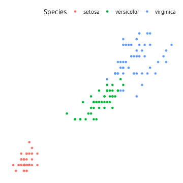
We are using the iris dataset using the three different species as groups/clusters.
iris %>%
  ggplot(aes(Petal.Length, Petal.Width, colour=Species))+
  geom_point()+
  theme_custom()
Base
First we start by using base functions.
Ellipse
Perhaps the easiest approach is drawing confidence ellipse. All points are not guaranteed to be inside the ellipse. The default level is 0.95. Increasing this includes more of the points, but the ellipses may get too large. The nice thing about this approach is that it is not strongly affected by outliers. This is well suited for clusters where points have a large spread and overlap a lot.
ggplot(data=iris, aes(Petal.Length, Petal.Width, colour=Species))+
  geom_point()+
  stat_ellipse(level=0.95)+
  theme_custom()
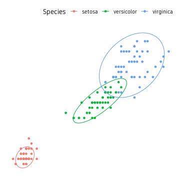
For most part, this is the easiest approach and good enough.
Convex hull
The outermost points in a point cloud can be connected to form a polygon referred to as the convex hull of a point cloud. The convex hull can be computed using the base function chull(). This can be used in a dplyr pipeline as shown below.
hull <- iris %>%
 group_by(Species) %>%
 slice(c(chull(Petal.Length, Petal.Width),
         chull(Petal.Length, Petal.Width)[1]))
The information to draw polygons around all three clusters is contained in the data.frame hull. The points and the polygons can be plotted as shown below.
ggplot()+
  geom_point(data=iris, aes(Petal.Length, Petal.Width, colour=Species))+
  geom_path(data=hull, aes(Petal.Length, Petal.Width, colour=Species))+
  theme_custom()
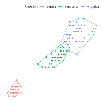
This is a good start, but it would be nicer if the edges of the polygon had smooth edges rather than sharp edges. While we could use some custom script to smooth it, the easier approach is to use from existing packages.
Density and contours
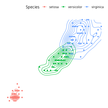
Before we move on, another idea from the base functions is to compute a 2D kernal density from the point cloud and draw countour lines.
iris %>%
  ggplot(aes(Petal.Length, Petal.Width, colour=Species))+
  geom_point()+
  geom_density_2d()+
  theme_custom()
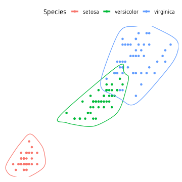
ggalt
geom_encircle
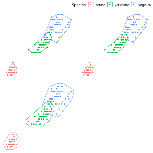
We use the function geom_encircle() from package ggalt to draw smoothed lines around clusters.
ggplot(data=iris, aes(Petal.Length, Petal.Width, colour=Species))+
  geom_point()+
  ggalt::geom_encircle(size=1.6)+
  theme_custom()
ggforce
Another useful package for marking clusters is ggforce. Below is a demonstration of four functions for marking clusters. The four functions are geom_mark_rect(), geom_mark_circle(), geom_mark_ellipse() and geom_mark_hull(). The shapes they create is self-explanatory.
p1 <- ggplot(data=iris, aes(Petal.Length, Petal.Width, colour=Species))+
  geom_point()+
  geom_mark_rect()+
  theme_custom()

p2 <- ggplot(data=iris, aes(Petal.Length, Petal.Width, colour=Species))+
  geom_point()+
  geom_mark_circle()+
  theme_custom()

p3 <- ggplot(data=iris, aes(Petal.Length, Petal.Width, colour=Species))+
  geom_point()+
  geom_mark_ellipse()+
  theme_custom()

p4 <- ggplot(data=iris, aes(Petal.Length, Petal.Width, colour=Species))+
  geom_point()+
  geom_mark_hull()+
  theme_custom()

ggpubr::ggarrange(p1, p2, p3, p4, nrow=2, ncol=2, common.legend=T)
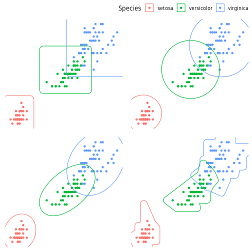
geom_mark_hull() has extra arguments to control concavity, radius and size (expand) of the hull shape. geom_mark_* functions also support an argument label to label the the marks. In this case, the plot legend can be turned off.
ggplot(data=iris, aes(Petal.Length, Petal.Width, colour=Species))+
  geom_point()+
  geom_mark_ellipse(aes(label=Species), label.colour="grey30")+
  theme_custom()+
  theme(legend.position="none")
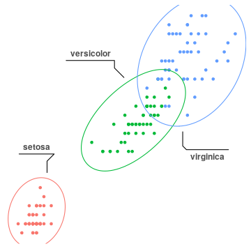
geom_mark_ellipse().
It is not necessary to mark all the groups. A particular group of interest can be marked alone.
ggplot()+
  geom_point(data=iris, aes(Petal.Length, Petal.Width))+
  geom_mark_ellipse(data=filter(iris, Species=="setosa"), aes(Petal.Length, Petal.Width, label=Species), label.colour="grey30", description="This is a brief description about this annotation.")+
  theme_custom()+
  theme(legend.position="none")
For more control over text annotation, see package ggrepel.
The ggforce package also has a function called geom_shape() to draw polygons but with some neat features. We can adjust the corner radius of the polygon to smooth the edges. We can also increase or decrease the overall size of the polygon. In this case, we use the convex hull object hull which we computed earlier.
p1 <- ggplot()+
  geom_point(data=iris, aes(Petal.Length, Petal.Width, colour=Species))+
  geom_shape(data=hull, aes(Petal.Length, Petal.Width, colour=Species), fill=NA)+
  theme_custom()
p2 <- ggplot()+
  geom_point(data=iris, aes(Petal.Length, Petal.Width, colour=Species))+
  geom_shape(data=hull, aes(Petal.Length, Petal.Width, colour=Species), fill=NA, radius=0.05)+
  theme_custom()
p3 <- ggplot()+
  geom_point(data=iris, aes(Petal.Length, Petal.Width, colour=Species))+
  geom_shape(data=hull, aes(Petal.Length, Petal.Width, colour=Species), fill=NA, radius=0.05, expand=0.04)+
  theme_custom()
ggpubr::ggarrange(p1, p2, p3, nrow=2, ncol=2, common.legend=T)
The package ggforce has many more cool features. You should check out their website.


Comments