Customising a ggplot2 plot using the theme function. In this post, we are going to explore how to adjust various ggplot plot elements. What can be adjusted, what they are called and how they can be adjusted.
First, load the packages that will be used. The extrafont package is used to import custom fonts and is completely optional.
library(ggplot2)
library(dplyr)
library(RColorBrewer)
library(Cairo)
library(ggpubr)

library(extrafont) # for custom font
loadfonts(device="win")
Base plot
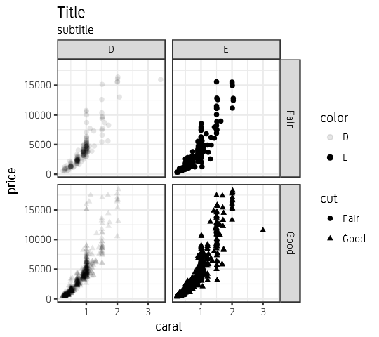
We create a basic sample plot to play around with.I am using the ‘diamonds’ datasets. The dataset is filtered to reduce the number of data points. Note that the pipe operator %>% from the magrittr package is used to connect subsequent commands. The default theme is set to theme_bw. The base_family="Gidole" only need to be set if adjusting the default font.
p <- diamonds %>%
  filter(cut=="Fair"|cut=="Good", color=="D"|color=="E") %>%
  droplevels() %>%
  ggplot(aes(carat, price, alpha=color, shape=cut))+
  geom_point()+
  labs(title="Title", subtitle="subtitle")+
  facet_grid(cut~color)+
  theme_bw(base_family="Gidole")
p
All non-data related plot elements are adjusted through the theme() function. All possible arguments to theme that can be adjusted can be inspected using args(theme). Explanations for these arguments are available through ?theme.
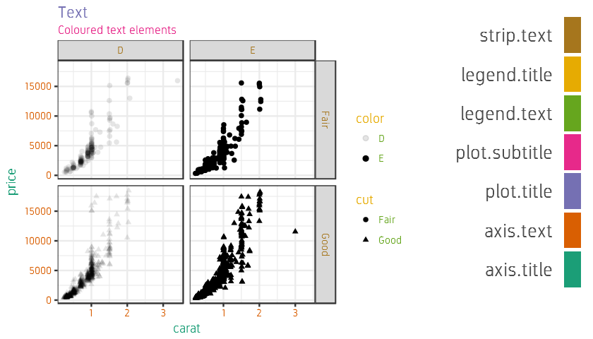
Text elements
First, we explore the text elements in the plot that can be adjusted. All text elements are adjusted through the element_text() function.
args(element_text)
function (family = NULL, face = NULL, colour = NULL, size = NULL,
          hjust = NULL, vjust = NULL, angle = NULL, lineheight = NULL,
          color = NULL, margin = NULL, debug = NULL, inherit.blank = FALSE)
Here, I am setting each text element to a unique colour so that it can be identified on out sample plot.
# change colour of text elements
cols <- brewer.pal(7, "Dark2")

p1 <- p +
  labs(title="Text", subtitle="Coloured text elements")+
  theme(axis.title=element_text(color=cols[1]),
  axis.text=element_text(color=cols[2]),
  plot.title=element_text(color=cols[3]),
  plot.subtitle=element_text(color=cols[4]),
  legend.text=element_text(color=cols[5]),
  legend.title=element_text(color=cols[6]),
  strip.text=element_text(color=cols[7]))
Here, I am creating a legend plot to be placed on the right side.
dfr <- data.frame(value=rep(1, 7), label=c("axis.title", "axis.text", "plot.title", "plot.subtitle", "legend.text", "legend.title", "strip.text"), stringsAsFactors=FALSE) %>%
  mutate(label=factor(label, levels=c("axis.title", "axis.text", "plot.title", "plot.subtitle", "legend.text", "legend.title", "strip.text")))

q <- ggplot(dfr, aes(x=label, y=value, fill=label))+
  geom_bar(stat="identity")+
  labs(x="", y="")+
  coord_flip()+
  scale_fill_manual(values=cols)+
  theme_minimal(base_size=20, base_family="Gidole")+
  theme(
    legend.position="none",
    axis.text.x=element_blank(),
    axis.ticks=element_blank(),
    panel.grid=element_blank())

ggarrange(p1, q, nrow=1, ncol=2, widths=c(0.7, 0.3))
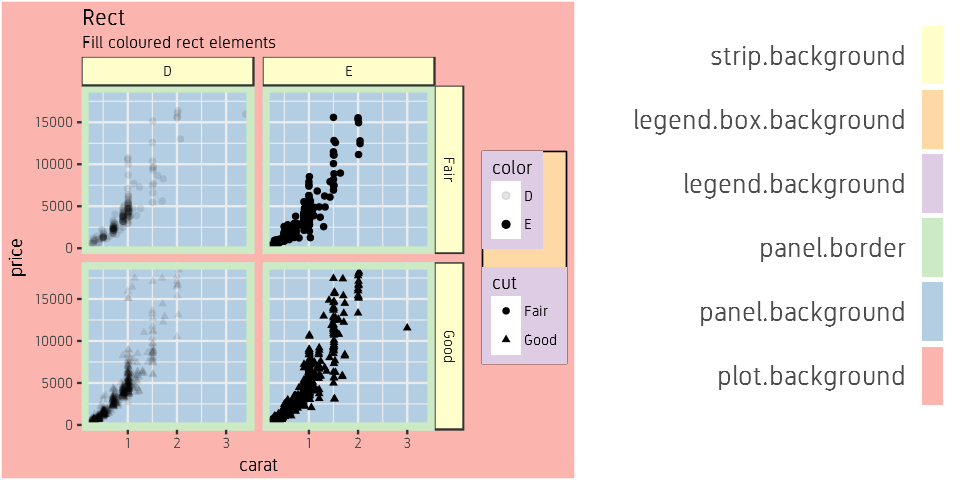
Rectangular elements
Now, we explore the rectangle elements. All rectangle elements are adjusted through the element_rect() function.
args(element_rect)
function (fill = NULL, colour = NULL, size = NULL, linetype = NULL,color = NULL, inherit.blank = FALSE)

# change fill colour of rectangular elements
cols <- brewer.pal(6, "Pastel1")

p1 <- p +
  labs(title="Rect", subtitle="Fill coloured rect elements")+
  theme(plot.background=element_rect(fill=cols[1]),
  panel.background=element_rect(fill=cols[2]),
  panel.border=element_rect(fill=NA, size=3, color=cols[3]),
  legend.background=element_rect(fill=cols[4]),
  legend.box.background=element_rect(fill=cols[5]),
  strip.background=element_rect(fill=cols[6]))
Now the legend.
dfr <- data.frame(value=rep(1, 6), label=c("plot.background", "panel.background", "panel.border", "legend.background", "legend.box.background", "strip.background"), stringsAsFactors=FALSE) %>%
  mutate(label=factor(label, levels=c("plot.background", "panel.background", "panel.border", "legend.background", "legend.box.background", "strip.background")))

q <- ggplot(dfr, aes(x=label, y=value, fill=label))+
  geom_bar(stat="identity")+
  labs(x="", y="")+
  coord_flip()+
  scale_fill_manual(values=cols)+
  theme_minimal(base_size=20, base_family="Gidole")+
  theme(
    legend.position="none",
    axis.text.x=element_blank(),
    axis.ticks=element_blank(),
    panel.grid=element_blank())

ggarrange(p1, q, nrow=1, ncol=2, widths=c(0.6, 0.4))
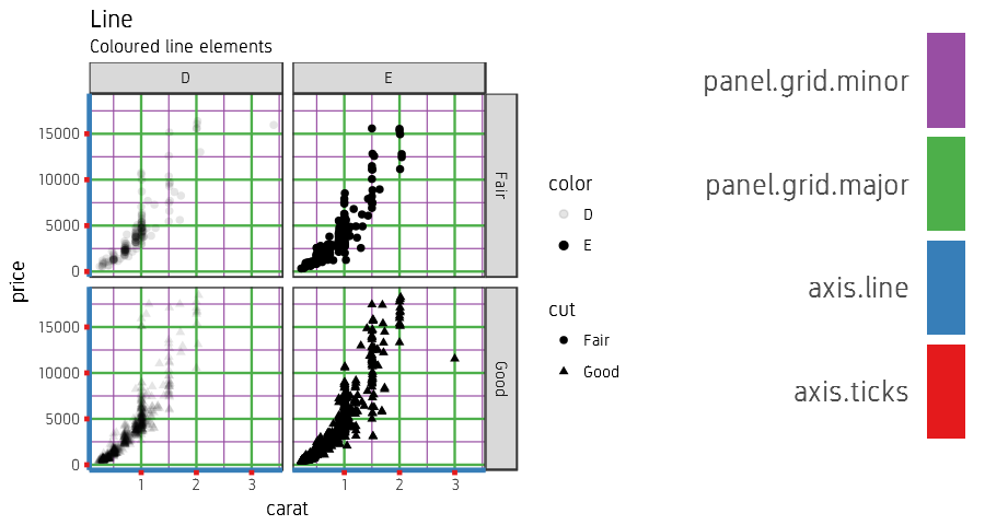
Line elements
Here we have the line elements. All line elements are adjusted through the element_line() function.
args(element_line)
function (colour = NULL, size = NULL, linetype = NULL, lineend = NULL, color = NULL, arrow = NULL, inherit.blank = FALSE)

# change line elements
cols <- brewer.pal(4, "Set1")

p1 <- p +
  labs(title="Line", subtitle="Coloured line elements")+
  theme(axis.ticks=element_line(colour=cols[1], size=1),
  axis.line=element_line(colour=cols[2], size=1),
  panel.grid.major=element_line(colour=cols[3]),
  panel.grid.minor=element_line(colour=cols[4]))
Now the legend.
dfr <- data.frame(value=rep(1, 4), label=c("axis.ticks", "axis.line", "panel.grid.major", "panel.grid.minor"), stringsAsFactors=FALSE) %>%
  mutate(label=factor(label, levels=c("axis.ticks", "axis.line", "panel.grid.major", "panel.grid.minor")))

q <- ggplot(dfr, aes(x=label, y=value, fill=label))+
  geom_bar(stat="identity")+
  labs(x="", y="")+
  coord_flip()+
  scale_fill_manual(values=cols)+
  theme_minimal(base_size=20, base_family="Gidole")+
  theme(
    legend.position="none",
    axis.text.x=element_blank(),
    axis.ticks=element_blank(),
    panel.grid=element_blank())

ggarrange(p1, q, nrow=1, ncol=2, widths=c(0.65, 0.35))
Margins and spacings
Margins are set using margin() and spacing is set using grid::unit().
Below shows the effect of increasing margins on the left and right of legend (red), legend.box (blue) and plot (green).
cols <- brewer.pal(4, "Pastel1")

p1 <- p + labs(title="Margin", subtitle="Default")
p2 <- p + theme(
  legend.background=element_rect(fill=cols[1]),
  legend.box.background=element_rect(fill=cols[2]),
  plot.background=element_rect(fill=cols[3]))+
  labs(title="Margin", subtitle="Default + Fill colour")

p3 <- p + theme(
  legend.margin=margin(r=20, l=20),
  legend.box.margin=margin(r=20, l=20),
  plot.margin=margin(r=20, l=20))+
  labs(title="Margin", subtitle="Increased margin")

p4 <- p + theme(
  legend.background=element_rect(fill=cols[1]),
  legend.box.background=element_rect(fill=cols[2]),
  plot.background=element_rect(fill=cols[3]),
  legend.margin=margin(r=20, l=20),
  legend.box.margin=margin(r=20, l=20),
  plot.margin=margin(r=20, l=20))+
  labs(title="Margin", subtitle="Increased margin + Fill colour")

ggarrange(p, p2, p3, p4, nrow=2, ncol=2)
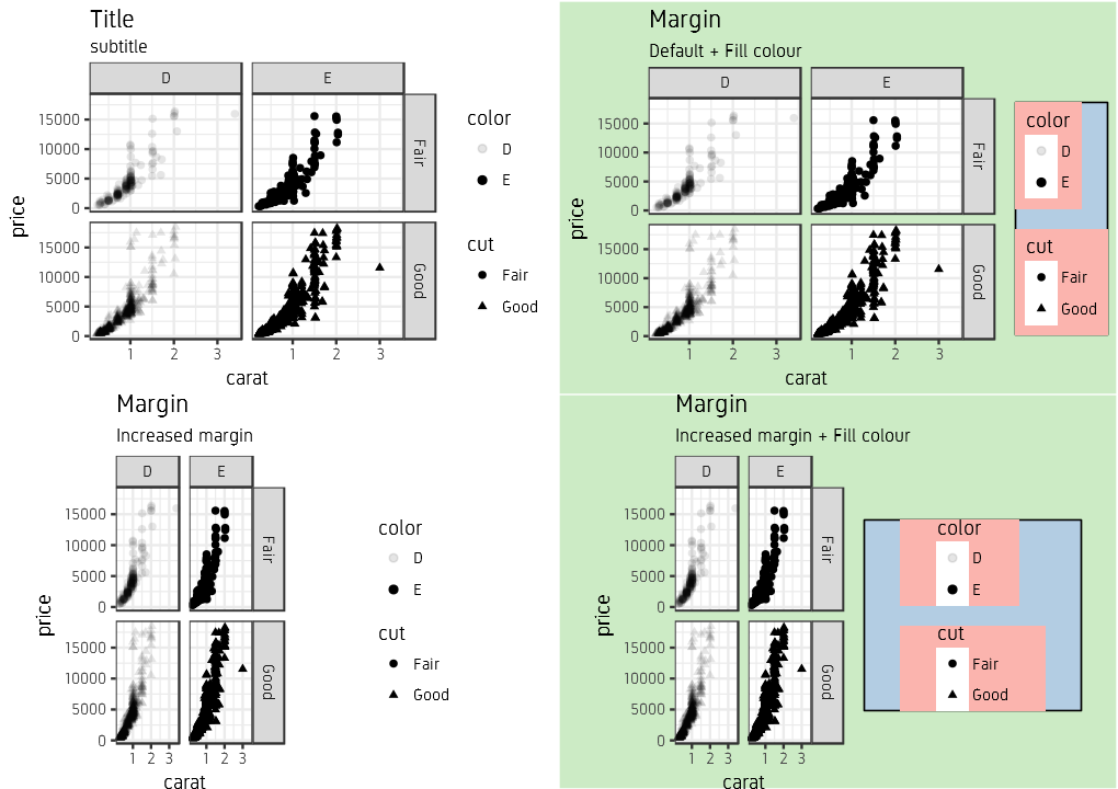
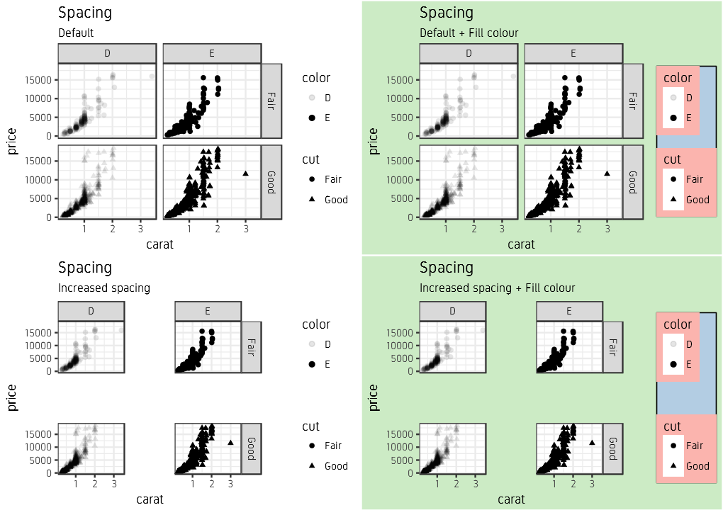
Left and right both shows the same effect of adjusting margins. Right is coloured. Below we adjust spacing.
cols <- brewer.pal(4, "Pastel1")

p1 <- p + labs(title="Spacing", subtitle="Default")

p2 <- p + theme(
  legend.background=element_rect(fill=cols[1]),
  legend.box.background=element_rect(fill=cols[2]),
  plot.background=element_rect(fill=cols[3]))+
  labs(title="Spacing", subtitle="Default + Fill colour")

p3 <- p + theme(
  legend.spacing=grid::unit(1, "cm"),
  legend.box.spacing=grid::unit(1, "cm"),
  panel.spacing=grid::unit(1.5, "cm"))+
  labs(title="Spacing", subtitle="Increased spacing")

p4 <- p + theme(
  legend.background=element_rect(fill=cols[1]),
  legend.box.background=element_rect(fill=cols[2]),
  plot.background=element_rect(fill=cols[3]),
  legend.spacing=grid::unit(1, "cm"),
  legend.box.spacing=grid::unit(1, "cm"),
  panel.spacing=grid::unit(1.5, "cm"))+
  labs(title="Spacing", subtitle="Increased spacing + Fill colour")

ggarrange(p1, p2, p3, p4, nrow=2, ncol=2)
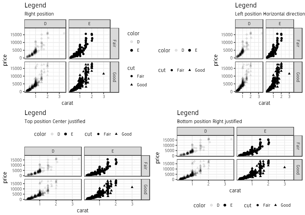
Position
Some of the plot elements can be moved around and repositioned. For example; legend.position moves the legend to the ‘left’, ‘right’, ‘top’,’bottom’ or ‘none’. legend.justification specifies how the legend is aligned horizontally, ie; ‘left’, ‘center’ etc. legend.direction specifies the layout of the legend, if it is ‘vertical’ or ‘horizontal’.
p1 <- p + theme(legend.position="right")+
                labs(title="Legend", subtitle="Right position")
p2 <- p + theme(legend.position="left", legend.direction="horizontal")+
                labs(title="Legend", subtitle="Left position Horizontal direction")
p3 <- p + theme(legend.position="top", legend.justification="center")+
                labs(title="Legend", subtitle="Top position Center justified")
p4 <- p + theme(legend.position="bottom", legend.justification="right")+
                labs(title="Legend", subtitle="Bottom position Right justified")

ggarrange(p1, p2, p3, p4, nrow=2, ncol=2)
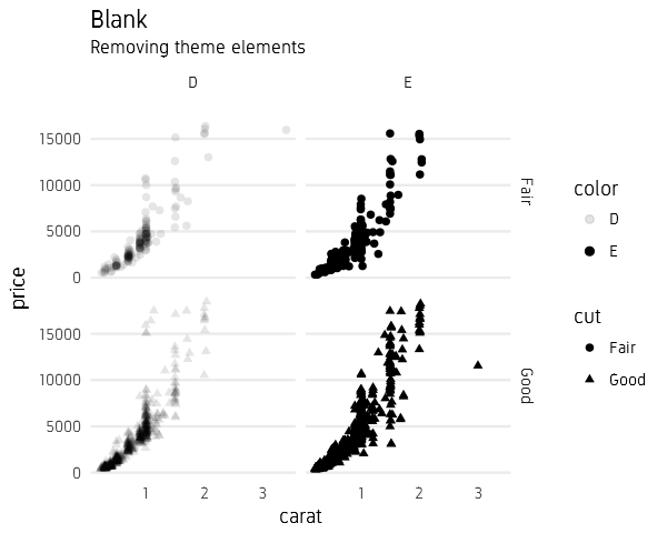
Remove elements
Any of the theme elements can be removed/not displayed by setting that argument to element_blank(). Here, I am creating a minimal looking plot by removing unnecessary elements.
p1 <- p +
  labs(title="Blank", subtitle="Removing theme elements")+
  theme(panel.border=element_blank(),
  panel.grid.major.x=element_blank(),
  panel.grid.minor=element_blank(),
  axis.ticks=element_blank(),
  strip.background=element_blank())

print(p1)
Saving themes
Any changes made to the ggplot2 theme elements can be saved for future use. There are at least two ways to do this.
One approach is simply to save it as a variable and apply it to a ggplot.
custom <- theme(panel.border=element_blank(),
  panel.grid.major.x=element_blank(),
  panel.grid.minor=element_blank(),
  axis.ticks=element_blank(),
  strip.background=element_blank())

p + custom
Another approach is to create a new theme function either from scratch or by modifying an existing theme. And then apply it as a theme function.
theme_custom <- function (basesize=14) {
    theme_bw(base_size=basesize) %+replace%
        theme(panel.border=element_blank(),
          panel.grid.major.x=element_blank(),
          panel.grid.minor=element_blank(),
          axis.ticks=element_blank(),
          strip.background=element_blank())
}

p + theme_custom()
Session
devtools::session_info()

Below is the session info showing R version and versions of all loaded packages.

Session info ---------------------------------------------------------------------
  setting  value
  version  R version 3.4.3 (2017-11-30)
  system   x86_64, mingw32
  ui       RStudio (1.1.442)
  language (EN)
  collate  English_United Kingdom.1252
  tz       Europe/Berlin
  date     2018-05-04

Packages -------------------------------------------------------------------------
  package      * version date       source
  assertthat     0.2.0   2017-04-11 CRAN (R 3.4.1)
  backports      1.1.2   2017-12-13 CRAN (R 3.4.3)
  base         * 3.4.3   2017-12-06 local
  bindr          0.1.1   2018-03-13 CRAN (R 3.4.3)
  bindrcpp     * 0.2     2017-06-17 CRAN (R 3.4.1)
  Cairo        * 1.5-9   2015-09-26 CRAN (R 3.4.0)
  cli            1.0.0   2017-11-05 CRAN (R 3.4.3)
  colorspace     1.3-2   2016-12-14 CRAN (R 3.4.1)
  compiler       3.4.3   2017-12-06 local
  cowplot        0.9.2   2017-12-17 CRAN (R 3.4.3)
  crayon         1.3.4   2017-09-16 CRAN (R 3.4.3)
  datasets     * 3.4.3   2017-12-06 local
  devtools       1.13.5  2018-02-18 CRAN (R 3.4.3)
  digest         0.6.15  2018-01-28 CRAN (R 3.4.3)
  dplyr        * 0.7.4   2017-09-28 CRAN (R 3.4.3)
  evaluate       0.10.1  2017-06-24 CRAN (R 3.4.1)
  extrafont    * 0.17    2014-12-08 CRAN (R 3.4.0)
  extrafontdb    1.0     2012-06-11 CRAN (R 3.4.0)
  gdtools      * 0.1.7   2018-02-27 CRAN (R 3.4.3)
  ggplot2      * 2.2.1   2016-12-30 CRAN (R 3.4.1)
  ggpubr       * 0.1.6   2017-11-14 CRAN (R 3.4.3)
  glue           1.2.0   2017-10-29 CRAN (R 3.4.3)
  graphics     * 3.4.3   2017-12-06 local
  grDevices    * 3.4.3   2017-12-06 local
  grid           3.4.3   2017-12-06 local
  gridExtra    * 2.3     2017-09-09 CRAN (R 3.4.1)
  gtable         0.2.0   2016-02-26 CRAN (R 3.4.1)
  htmltools      0.3.6   2017-04-28 CRAN (R 3.4.1)
  knitr          1.20    2018-02-20 CRAN (R 3.4.3)
  labeling       0.3     2014-08-23 CRAN (R 3.4.0)
  lazyeval       0.2.1   2017-10-29 CRAN (R 3.4.3)
  magrittr     * 1.5     2014-11-22 CRAN (R 3.4.1)
  memoise        1.1.0   2017-04-21 CRAN (R 3.4.1)
  methods      * 3.4.3   2017-12-06 local
  munsell        0.4.3   2016-02-13 CRAN (R 3.4.1)
  pillar         1.2.1   2018-02-27 CRAN (R 3.4.3)
  pkgconfig      2.0.1   2017-03-21 CRAN (R 3.4.1)
  plyr           1.8.4   2016-06-08 CRAN (R 3.4.1)
  pophelper      2.2.6   2018-05-01 local
  purrr          0.2.4   2017-10-18 CRAN (R 3.4.3)
  R6             2.2.2   2017-06-17 CRAN (R 3.4.1)
  RColorBrewer * 1.1-2   2014-12-07 CRAN (R 3.4.0)
  Rcpp           0.12.16 2018-03-13 CRAN (R 3.4.3)
  reshape2       1.4.3   2017-12-11 CRAN (R 3.4.3)
  rlang          0.2.0   2018-02-20 CRAN (R 3.4.3)
  rmarkdown      1.9     2018-03-01 CRAN (R 3.4.3)
  rprojroot      1.3-2   2018-01-03 CRAN (R 3.4.3)
  rsconnect      0.8.8   2018-03-09 CRAN (R 3.4.3)
  rstudioapi     0.7     2017-09-07 CRAN (R 3.4.3)
  Rttf2pt1       1.3.6   2018-02-22 CRAN (R 3.4.3)
  scales         0.5.0   2017-08-24 CRAN (R 3.4.1)
  stats        * 3.4.3   2017-12-06 local
  stringi        1.1.7   2018-03-12 CRAN (R 3.4.3)
  stringr      * 1.3.0   2018-02-19 CRAN (R 3.4.3)
  svglite        1.2.1   2017-09-11 CRAN (R 3.4.3)
  tibble         1.4.2   2018-01-22 CRAN (R 3.4.3)
  tidyr          0.8.0   2018-01-29 CRAN (R 3.4.3)
  tools          3.4.3   2017-12-06 local
  utf8           1.1.3   2018-01-03 CRAN (R 3.4.3)
  utils        * 3.4.3   2017-12-06 local
  withr          2.1.1   2017-12-19 CRAN (R 3.4.3)
  yaml           2.1.18  2018-03-08 CRAN (R 3.4.3)


Comments