Multiple Statistical Testing

In a standard statistical test, one assumes a null hypothesis, performs a statistical test and computes a p-value. The estimated p-value is compared to a predetermined threshold (usually 0.05). If the estimated p-value is greater than 0.05 (say 0.2), it means that there is a 20% chance of obtaining the current result if the null hypothesis is true. Since we decided our threshold as 5%, the 20% is too high to reject the null hypothesis and we accept the null hypothesis. Now, if the estimated p-value was less than 0.05 (say 0.02), there is a 2% probability of obtaining the observed result if the null hypothesis is true. Since 2% is a very low probability and it is below our threshold of 5%, we reject the null hypothesis and accept an alternative hypothesis.

The 5% threshold, although giving us high confidence, is an arbitrary value and does not absolutely guarantee an outcome. There is still the possibility that we are wrong 5% of the time. This is known as the probability of a Type I error. A Type I error occurs when a researcher falsely concludes that an observed difference is real, when in fact, there is no difference.

That was the story of a single statistical test. With large data, it is common for data analysts to do multiple statistical tests on the same data. Similar to a single test, each test in a multiple test has the 5% Type 1 error rate. And this accumulates for the number of tests.

The probability of accumulating type I (t1) errors can be shown as below:

    P(making an t1 error) = a
    P(not making a t1 error) = 1-a
    P(not making a t1 error in m tests) = (1-a)^m
    P(not making at least 1 t1 error in m tests) = 1-(1-a)^m

    Probability of a t1 error with one test (m=1):
    1 - (1 - 0.05)^1
    0.05

    Probability of a t1 error with 10 tests (m=10):
    1 - (1 - 0.05)^10
    0.40

So, for 10 tests, there is a 40% chance of observing at least one significant result even if there are none. If 100 genes are tested, 5% (5 genes) could be found to be significant by chance even if they are not. In datasets such as RNA-seq data where thousands of genes are tested, the type I error rate gets inflated massively. This is the reason why p-values from multiple testing needs to be corrected.

Methods for dealing with multiple testing usually involves adjusting p-value threshold in some way, so that the probability of observing at least one significant result due to chance remains below a desired significance level.

There are several categories of methods to controlling Type I errors:  Per Comparison Error Rate (PCER), Per Family Error Rate (PFER), Family-Wise Error Rate (FWER), False Discovery Rate (FDR), Positive False Discovery (pFDR) etc. We will only consider two categories of methods to correcting for multiple testing, namely, controlling the family-wise error rate (FWER) and controlling the false discovery rate (FDR).

Control Family-wise error rate (FWER)

Bonferroni correction

The classical single-step approach and the simplest method is the Bonferroni correction. It is also the most stringent method. All tested p-values are multiplied by the total number of tests.

    Corrected p-value = p-value * num_tests

Example:

    Let n=1000, p-value threshold=0.05
    Rank Gene p-value
    1 A 0.00002
    2 B 0.00004
    3 C 0.00009

    Correction:
    GeneA p-value = 0.00002 * 1000 = 0.02 (significant)
    GeneB p-value = 0.00004 * 1000 = 0.04 (significant)
    GeneC p-value = 0.00009 * 1000 = 0.09 (not significant)

Using a p-value of 0.05 means there is a 5% or less chance of 1 test being a false positive. Another definition is to expect 0.05 genes to be significant by chance. Using the Bonferroni correction brings the error probability back to 5% as shown below.

    1-(1-(a/m))^m
    1 - (1 - 0.05/10)^10
    0.05

The Bonferroni correction has a few drawbacks of its own. It may be suitable when we want to avoid even a single false positive in the results. But in most cases, this is too extreme such that false negatives (type II errors) may be inflated. Thus truly important differences may be deemed non-significant.

Bonferroni step-down (Holm)

This is a modified Bonferroni method using sequential step-down and it is slightly less stringent than the Bonferroni method.

1. Take the p-value of each gene and rank them from the smallest to the largest.

2. Multiply the first p-value by the number of genes present in the gene list: if the end value is less than 0.05, the gene is significant. ` Corrected P-value= p-value * n`

3. Multiply the second p-value by the number of genes less 1: ` Corrected P-value= p-value * (n-1)`

4. Multiply the third p-value by the number of genes less 2: ` Corrected P-value= p-value * (n-2)` Follow that sequence until no gene is found to be significant.

Example:

    Let n=1000, p-value threshold=0.05
    Rank Gene p-value
    1 A 0.00002
    2 B 0.00004
    3 C 0.00009

    Correction:
    GeneA p-value = 0.00002 * 1000 = 0.02 (significant)
    GeneB p-value = 0.00004 * 999 = 0.039 (significant)
    GeneC p-value = 0.00009 * 998 = 0.0898 (not significant)

Controlling FWER is generally too extreme and appropriate only in situations where a researcher does not want ANY false positives at the risk of missing out few true positives. A more relevant quantity to control is the FDR.

Control False discovery rate (FDR)

Controlling for False discovery rate (FDR) is currently the preferred approach to account for multiple testing. FDR sets the proportion of discoveries (significant results) that are actually false positives. For example, one could set the FDR to 0.05 and all tested p-values are adjusted. Of the tests that are still significant (below 0.05), 5% could be false positives. Depending on the situation, FDR could be set to 5%, 10%, 15% etc. The False Discovery Rate (FDR) control was developed by Benjamini and Hochberg in 1995.

Benjamini-Hochberg

This correction is the least stringent  and the most powerful option. Here is how it works:

Here is how it works:

1. Rank the p-value of each gene in order from the smallest to the largest.
2. Multiply the largest p-value by the number of genes in the test.
3. Take the second largest p-value and multiply it by the total number of genes in gene list divided by its rank. If less than 0.05, it is significant. ` Corrected p-value = p-value * (n/n-1)`
4. Take the third p-value and proceed as in step 3: ` Corrected p-value = p-value * (n/n-2)`

Example:

    Let n=1000, p-value threshold=0.05
    Rank Gene p-value
    1000 A 0.1
    999 B 0.04
    998 C 0.01

    Correction:
    GeneA P-value > 0.05 => gene D (not significant)
    GeneB P-value = (1000/999) * 0.04 = 0.04004 (significant)
    GeneC P-value = (1000/998) * 0.01 = 0.01002 (significant)

Practical example

We try out some examples of p-value correction with randomly generated data in R. We use the function p.adjust() from stats package and mt.rawp2adjp() from the multtest package.

We generate 10,000 random raw p-values between 0.00001 and 0.01. We assume these are p-values generated from 10,000 statistical tests. Since all p-values are below the threshold of 0.05, we will call this set the low set. Now we correct this dataset for multiple testing in R using six different methods: Benjamini-Hochberg (BH), Hommel, Benjamini-Yekutieli (BY), Holm, SidakSD and Bonferroni (B). The tests are roughly ordered in the level of stringency from least stringent to most stringent.

library(Cairo)
library(ggplot2)
library(tidyr)
library(dplyr)
library(multtest)

textcol <- "grey30"

#create a vector of random p-values
df1 <- data.frame(num=as.character(1:10000), 
Raw=runif(n = 10000, min=0.00001, max=0.01))

#create a dataframe of adjusted p-values
df1 <- df1 %>%
mutate(Holm=p.adjust(Raw, method="holm")) %>%
mutate(Hommel=p.adjust(Raw, method="hommel")) %>%
mutate(Bonferroni=p.adjust(Raw, method="bonferroni")) %>%
mutate(BenjaminiHochberg=p.adjust(Raw, method="BH")) %>%
mutate(BenjaminiYekutieli=p.adjust(Raw, method="BY")) %>%
mutate(SidakSD=mt.rawp2adjp(Raw, proc="SidakSD")$adjp[, 2])

df2 <- df1 %>% gather(key=method, value=measure, -num) %>%
mutate(method=factor(method, levels=c("Raw", "BenjaminiHochberg", "Hommel", "BenjaminiYekutieli", 
"Holm", "SidakSD", "Bonferroni"))) %>%
mutate(sig=ifelse(measure<0.05, "significant", "not-significant")) %>%
mutate(sig=factor(sig, levels=c("significant", "not-significant")))

# scatterplot
p <- ggplot(df2, aes(x=method, y=measure, colour=sig))+
#geom_point(alpha=0.8)+
geom_boxplot(alpha=0.8, size=0.25, position="identity", outlier.size=1)+
geom_hline(yintercept=0.05, colour=textcol, size=0.6, alpha=0.4, linetype="21")+
coord_flip()+
xlab("")+
ylab(expression( italic(p)-value))+
labs(caption="Boxplots showing 10,000 random raw p-values (0.00001 - 0.01) and six methods of multiple testing correction.")+
scale_colour_manual(values=c("#66c2a5", "#fc8d62"), guide=guide_legend(nrow=1))+
theme_bw(base_size=10)+
theme(
legend.position="top", 
legend.direction="horizontal", 
legend.justification="right", 
legend.title=element_blank(), 
legend.margin=margin(0, 4, -10, 0), 
legend.text=element_text(colour=textcol, size=6, face="plain"), 
legend.key.size=grid::unit(0.25, "cm"), 
strip.background=element_rect(colour="white", fill="grey90"), 
strip.text=element_text(face="bold"), 
axis.text.x=element_text(size=9, colour=textcol), 
axis.text.y=element_text(vjust=0.2, colour=textcol), 
axis.title=element_text(colour=textcol, size=8.5), 
axis.ticks=element_blank(), 
plot.title=element_text(colour=textcol, hjust=0, size=13, face="bold"), 
#plot.subtitle=element_text(colour=textcol, hjust=0, vjust=-1), 
plot.caption=element_text(colour=textcol, hjust=0, size=5, lineheight=-1), 
plot.margin=margin(10, 10, 5, 10), 
panel.grid=element_line(colour="grey99"), 
panel.border=element_blank())

ggsave("pval-scatterplot-low.png", p, height=6, width=13, units="cm", dpi=300, type="cairo")

Boxplots showing 10,000 raw p-values between 0.00001 and 0.01 and corrected p-values using six methods. Data is shown as boxplots. Central vertical line indicates median and points indicate outliers. Dotted line across all data denotes the significance threshold of 0.05. Significant data is coloured in green and non-significant data is coloured in red.

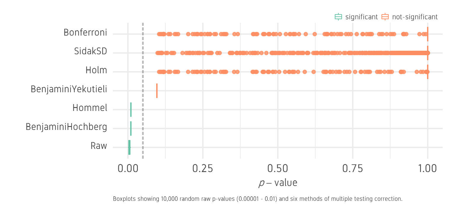
We see that BH and Hommel correction keep all 10,000 p-values below the significance threshold of 0.05. BY is close but not significant. BY values can be made significant by raising the FDR from 5% to 12% or so. Holm, Sidak and B correct aggressively and most p-values are insignificant.

Now we try the same idea but start with a set of p-values that are above and below the threshold of 0.05. We generate 10,000 random raw p-values between 0.00001 and 0.1. We will call this the lowhigh set.

#create a vector of random p-values
df1 <- data.frame(num=as.character(1:10000), 
  Raw=runif(n = 10000, min=0.00001, max=0.1))

Boxplots showing 10,000 raw p-values between 0.00001 and 0.1 and corrected p-values using six methods. Data is shown as boxplots. Central vertical line indicates median and points indicate outliers. Dotted line across all data denotes the significance threshold of 0.05. Significant data is coloured in green and non-significant data is coloured in red.

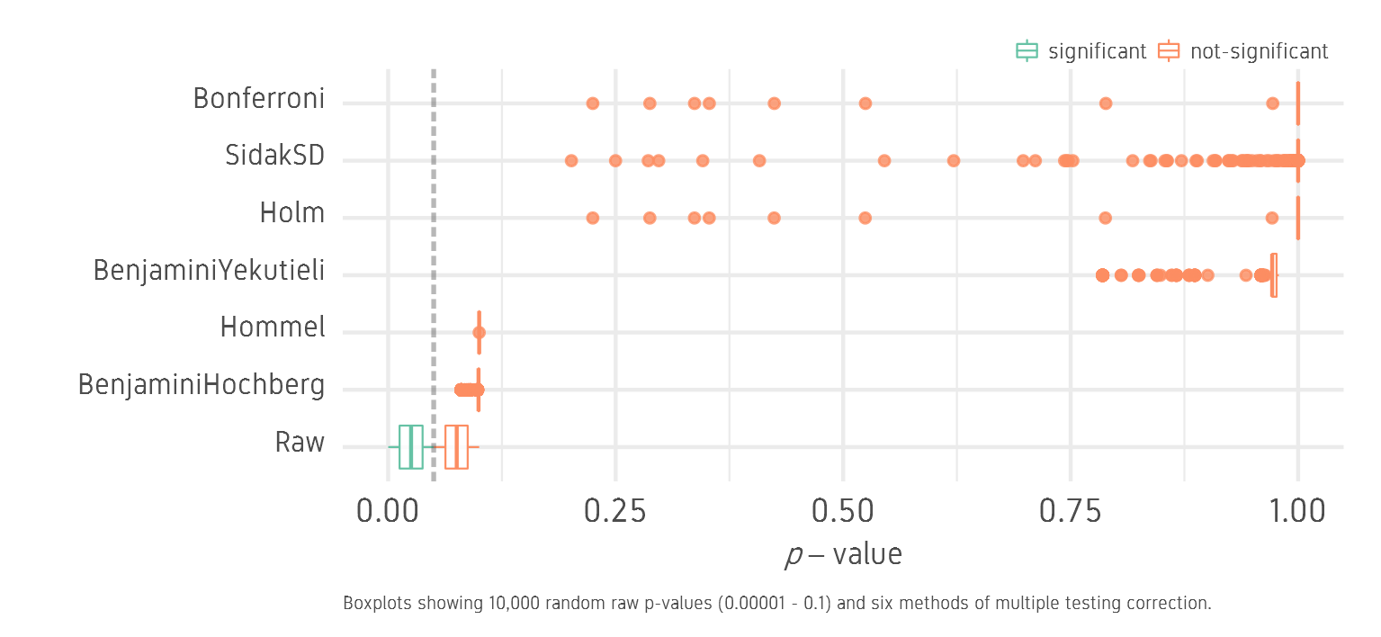
We see that the raw values are distributed below and above the 0.05 threshold. All correction methods push all values above the 0.05 threshold and none of the tests is significant.

So the starting distribution of p-values certainly has an effect on the outcome of the corrected p-values. Another critical factor is the number of samples/number of tests. The less the number of starting p-values, the less aggressive will be the correction. To demonstrate that, we generate a low set and a lowhigh set, but for each, we will generate five different sets of starting number (n=10,100,1000,10000,100000). Corrections using 100,000 data points can take a few minutes.

dlist <- list(length=5)
vec <- c(10, 100, 1000, 10000, 100000)
for(i in 1:length(vec))
{
  print(vec[i])
  #create a dataframe of adjusted p-values
  dlist[[i]] <- data.frame(num=as.character(1:vec[i]), Raw=runif(n = vec[i], min=0.00001, max=0.01)) %>%
  mutate(Holm=p.adjust(Raw, method="holm")) %>%
  mutate(Hommel=p.adjust(Raw, method="hommel")) %>%
  mutate(Bonferroni=p.adjust(Raw, method="bonferroni")) %>%
  mutate(BenjaminiHochberg=p.adjust(Raw, method="BH")) %>%
  mutate(BenjaminiYekutieli=p.adjust(Raw, method="BY")) %>%
  mutate(SidakSD=mt.rawp2adjp(Raw, proc="SidakSD")$adjp[, 2]) %>%
  gather(key=method, value=measure, -num) %>%
  mutate(method=factor(method, levels=c("Raw", "BenjaminiHochberg", "Hommel", "BenjaminiYekutieli", 
  "Holm", "SidakSD", "Bonferroni"))) %>%
  mutate(sig=ifelse(measure<0.05, "significant", "not-significant")) %>%
  mutate(sig=factor(sig, levels=c("significant", "not-significant"))) %>%
  mutate(n=paste0("n=", vec[i]))
}

df3 <- bind_rows(dlist) %>%
  mutate(n=factor(n))

# scatterplot
p <- ggplot(df3, aes(x=method, y=measure, colour=sig))+
  geom_boxplot(alpha=0.8, size=0.25, position="identity", outlier.size=0.85)+
  geom_hline(yintercept=0.05, colour=textcol, size=0.4, alpha=0.4, linetype="21")+
  coord_flip()+
  facet_wrap(~n, nrow=5)+
  xlab("")+
  ylab(expression( italic(p)-value))+
  labs(caption="Boxplots showing raw p-values and six adjustment methods using five different number of tests (n).")+
  scale_colour_manual(values=c("#66c2a5", "#fc8d62"), guide=guide_legend(nrow=1))+
  theme_bw(base_size=10)+
  theme(
  legend.position="top", 
  legend.direction="horizontal", 
  legend.justification="right", 
  legend.title=element_blank(), 
  legend.margin=margin(0, 4, -10, 0), 
  legend.text=element_text(colour=textcol, size=6, face="plain"), 
  legend.key.size=grid::unit(0.25, "cm"), 
  strip.background=element_rect(colour="white", fill="grey96"), 
  strip.text=element_text(face="bold", size=6, lineheight=0.4), 
  axis.text.x=element_text(size=6.5, colour=textcol), 
  axis.text.y=element_text(size=6.5, vjust=0.2, colour=textcol), 
  axis.title=element_text(colour=textcol, size=8), 
  axis.ticks=element_blank(), 
  plot.title=element_text(colour=textcol, hjust=0, size=13, face="bold"), 
  plot.caption=element_text(colour=textcol, hjust=0, size=4, lineheight=-1), 
  plot.margin=margin(10, 10, 5, 10), 
  panel.grid.major=element_line(colour="grey94", size=0.25), 
  panel.grid.minor=element_line(colour="grey96", size=0.15), 
  panel.border=element_blank())

ggsave("pval-n-scatterplot-low.png", p, height=13, width=9, units="cm", dpi=300, type="cairo")

Boxplots showing 10,000 raw p-values between 0.00001 and 0.01 and corrected p-values using six methods and six different number of tests. Data is shown as boxplots. Central vertical line indicates median and points indicate outliers. Dotted line across all data denotes the significance threshold of 0.05. Significant data is colored in green and non-significant data is coloured in red.

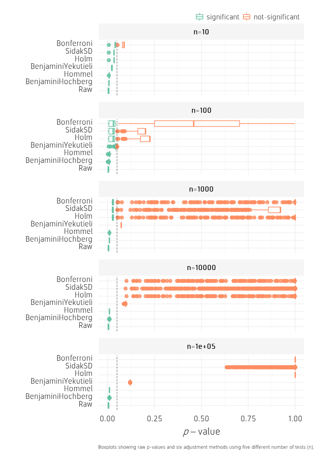
For the low set, as n increases from 10 to 100000, BH and Hommel methods keep all values below 0.05, while other methods drastically push the p-values further out towards 1. BY finds a compromise by keeping p-values low and significance can be achieved by increasing FDR.

Boxplots showing 10,000 raw p-values between 0.00001 and 0.1 and corrected p-values using six methods and six different number of tests. Data is shown as boxplots. Central vertical line indicates median and points indicate outliers. Dotted line across all data denotes the significance threshold of 0.05. Significant data is colored in green and non-significant data is coloured in red.

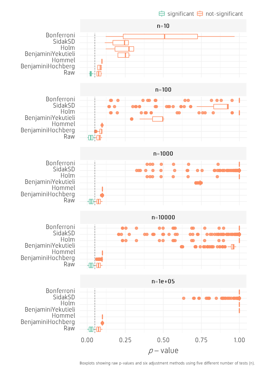
For the lowhigh set, the corrections seem to be even stronger pushing the corrected p-values higher than 0.05 with all methods and all n values.

Conclusion

As a general guide, multiple testing may not be necessary for exploratory analyses for hypothesis generation. FDR control may be suitable for exploratory analyses or screening to minimise false positives for further investigation. FWER control may be necessary for endpoint confirmatory analyses to absolutely eliminate any false positives.

In conclusion, when performing multiple statistical tests on the same data, it is important to correct the resulting p-values. Controlling for FDR is the more preferred way to adjust p-values. The most popular method at least for genomics is the Benjamini-Hochberg.

References

1. ETH multiple testing guide

2. Biostathandbook multiple comparison

3. Benjamini, Y., & Hochberg, Y. (1995). Controlling the false discovery rate: a practical and powerful approach to multiple testing. Journal of the royal statistical society. Series B (Methodological), 289-300.

4. Pollard, K. S., Dudoit, S., & van der Laan, M. J. (2005). Multiple testing procedures: the multtest package and applications to genomics. In Bioinformatics and computational biology solutions using R and bioconductor (pp. 249-271). Springer New York.

5. Bender, R., & Lange, S. (2001). Adjusting for multiple testing—when and how?. Journal of clinical epidemiology, 54(4), 343-349.

6. Noble, W. S. (2009). How does multiple testing correction work?. Nature biotechnology, 27(12), 1135-1137.

7. Reiner, A., D. Yekutieli and Y. Benjamini. (2003). Identifying differentially expressed genes using false discovery rate controlling procedures. Bioinformatics 19: 368-375.

Back to top ↑