Install tomahawk from here. Following commands are run on the Linux command-line.
Thinning VCF
For LD computation, pairwise comparisons are performed between all SNPs, therefore it is essential to thin down the number of SNPs. My dataset has about 18 million SNPs. My aim is to bring it down to 20,000 or so. Use vcftools to thin down a VCF file.
vcftools --vcf snp.vcf --recode --recode-INFO-all --thin 50000 --out "snp-thin"

VCFtools - 0.1.15
(C) Adam Auton and Anthony Marcketta 2009

Parameters as interpreted:
        --vcf snp.vcf
        --recode-INFO-all
        --thin 50000
        --out snp-thin
        --recode

After filtering, kept 64 out of 64 Individuals
Outputting VCF file...
After filtering, kept 26205 out of a possible 18793942 Sites
Run Time = 135.00 seconds

mv "snp-thin.recode.vcf" "snp-thin.vcf"
The argument --thin 50000 means to keep 1 SNP every 50,000 bases. Depending on the number of SNPs in the VCF file, you want to increase or decrease this. I am aiming for about 20,000 or so SNPs in the thinned file.
VCF to BCF
Convert VCF to BCF.
bcftools view snp.vcf -O b -o snp.bcf
Tomahawk
Instructions on using tomahawk is detailed here. Convert BCF to the tomahawk format. Import filters filter out sites with missingness > 20% and HW p-value < 0.001.
tomahawk import -i snp.bcf -o snp -m 0.2 -h 0.001
Tomahawk is used to compute LD.
Arguments: -u (unphased), -d (progress), -f (fast computation), -i (input file), -o (output file name prefix), -r (min R2 cut-off). See tomahawk help for more descriptions.
tomahawk calc -udfi snp.twk -o snp -a 5 -r 0.1 -P 0.1 -C 1 -t 1
The .two output is binary and needs to be exported to a text file. The -I arguments restricts the output to a specified chromosome. So, -I chr1 (UCSC) of -I 1 (Ensembl) exports only chromosome 1. It is probably better to have separate files for each chromosome as the files are a more managable size to read into R. The LD metrics are computed between SNPs within chromosomes anyway.
tomahawk view -i snp.two > snp.ld
tomahawk view -i snp.two -I 1 > snp-1.ld
Plotting
Now we move into R. First we load some libraries and define some plotting functions to be used later.
# load libraries
library(dplyr)
library(ggplot2)

# define plotting functions
#' @title plotPairwiseLD
#' @description Plots R2 heatmap across the chromosome (like Haploview)
#' @param dfr A data.frame with minimum CHROM_A, POS_A, CHROM_B, POS_B and R2.
#' An output from tomahawk works.
#' @param chr A chromosome name.
#' @param xlim A two number vector specifying min and max x-axis limits. Any one or both can be defaulted by specifying NA.
#' @param ylim A two number vector specifying min and max y-axis limits. Any one or both can be defaulted by specifying NA.
#' @param minr2 A value between 0 and 1. All SNPs with R2 value below this
#' value is excluded from plot.
#'
plotPairwiseLD <- function(dfr, chr, xlim = c(NA, NA), ylim = c(NA, NA), minr2) {
  if (missing(dfr)) stop("Input data.frame 'dfr' missing.")

  if (!missing(chr)) {
    ld <- filter(ld, CHROM_A == get("chr") & CHROM_B == get("chr"))
  }
  ld <- filter(ld, POS_A < POS_B)

  if (!missing(minr2)) {
    ld <- filter(ld, R2 > get("minr2"))
  }

  ld <- ld %>% arrange(R2)

  ld$x <- ld$POS_A + ((ld$POS_B - ld$POS_A) / 2)
  ld$y <- ld$POS_B - ld$POS_A
  ld$r2c <- cut(ld$R2, breaks = seq(0, 1, 0.2), labels = c(
    "0-0 - 0.2", "0.2 - 0.4",
    "0.4 - 0.6", "0.6 - 0.8",
    "0.8 - 1.0"
  ))
  ld$r2c <- factor(ld$r2c, levels = rev(c(
    "0-0 - 0.2", "0.2 - 0.4",
    "0.4 - 0.6", "0.6 - 0.8",
    "0.8 - 1.0"
  )))

  ggplot(ld, aes(x = x, y = y, col = r2c)) +
    geom_point(shape = 20, size = 0.1, alpha = 0.8) +
    scale_color_manual(values = c("#ca0020", "#f4a582", "#d1e5f0", "#67a9cf", "#2166ac")) +
    scale_x_continuous(limits = xlim) +
    scale_y_continuous(limits = ylim) +
    guides(colour = guide_legend(title = "R2", override.aes = list(shape = 20, size = 8))) +
    labs(x = "Chromosome (Bases)", y = "") +
    theme_bw(base_size = 14) +
    theme(
      panel.border = element_blank(),
      axis.ticks = element_blank()
    ) %>%
    return()
}


#' @title plotDecayLD
#' @description Plots R2 heatmap across the chromosome (like Haploview)
#' @param dfr A data.frame with minimum CHROM_A, POS_A, CHROM_B, POS_B and R2.
#' An output from tomahawk works.
#' @param chr A chromosome name.
#' @param xlim A two number vector specifying min and max x-axis limits. Any one or both can be defaulted by specifying NA.
#' @param ylim A two number vector specifying min and max y-axis limits.  Any one or both can be defaulted by specifying NA.
#' @param avgwin An integer specifying window size. Mean R2 is computed within windows.
#' @param minr2 A value between 0 and 1. All SNPs with R2 value below this
#' value is excluded from plot.
#'
plotDecayLD <- function(dfr, chr, xlim = c(NA, NA), ylim = c(NA, NA), avgwin = 0, minr2) {
  if (missing(dfr)) stop("Input data.frame 'dfr' missing.")

  if (!missing(chr)) {
    ld <- filter(ld, CHROM_A == get("chr") & CHROM_B == get("chr"))
  }
  ld <- filter(ld, POS_A < POS_B)

  if (!missing(minr2)) {
    ld <- filter(ld, R2 > get("minr2"))
  }

  ld <- ld %>% arrange(R2)

  ld$dist <- ld$POS_B - ld$POS_A

  if (avgwin > 0) {
    ld$distc <- cut(ld$dist, breaks = seq(from = min(ld$dist), to = max(ld$dist), by = avgwin))
    ld <- ld %>%
      group_by(distc) %>%
      summarise(dist = mean(dist), R2 = mean(R2))
  }

  ggplot(ld, aes(x = dist, y = R2)) +
    geom_point(shape = 20, size = 0.15, alpha = 0.7) +
    geom_smooth() +
    scale_x_continuous(limits = xlim) +
    scale_y_continuous(limits = ylim) +
    labs(x = "Distance (Bases)", y = expression(LD ~ (r^{
      2
    }))) +
    theme_bw(base_size = 14) +
    theme(
      panel.border = element_blank(),
      axis.ticks = element_blank()
    ) %>%
    return()
}
Then we read the file.
ld <- read.delim("snp.ld", sep="\t", comment.char="#")
The output looks like below:
> head(ld)
  FLAG CHROM_A   POS_A CHROM_B   POS_B   REF_REF      REF_ALT   ALT_REF
1   10       1     359       1  100777 103.00000 8.526513e-14  5.000000
2   10       1  100777       1     359 103.00000 8.526513e-14  5.000000
3    2       1     359       1  452615  97.48765 5.512354e+00 10.512354
4    2       1  452615       1     359  97.48765 5.512354e+00 10.512354
5    6       1     359       1 1454410  49.07769 5.392231e+01  1.922308
6    6       1 1454410       1     359  49.07769 5.392231e+01  1.922308
    ALT_ALT          D    Dprime         R        R2            P ChiSqModel
1 20.00000 0.12573242 1.0000000 0.8734775 0.7629629 4.440203e-19   2.296495
2 20.00000 0.12573242 1.0000000 0.8734775 0.7629629 4.440203e-19   2.296495
3 14.48765 0.08266716 0.6574848 0.5742982 0.3298184 5.573234e-08   1.993300
4 14.48765 0.08266716 0.6574848 0.5742982 0.3298184 5.573234e-08   1.993300
5 23.07769 0.06280179 0.8070154 0.3235735 0.1046998 1.876711e-04   7.703488
6 23.07769 0.06280179 0.8070154 0.3235735 0.1046998 1.876711e-04   7.703488
  ChiSqTable
1   97.65926
2   97.65926
3   42.21675
4   42.21675
5   13.40157
6   13.40157
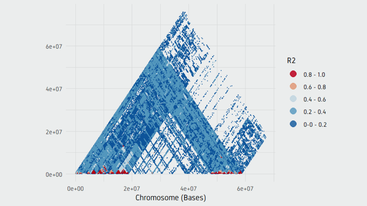
Plot pairwise LD plot.
plotPairwiseLD(ld)
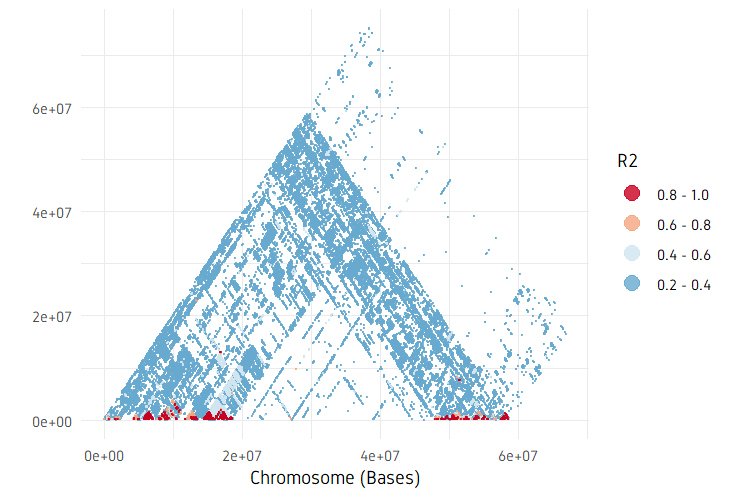
plotPairwiseLD(ld, minr2=0.2)
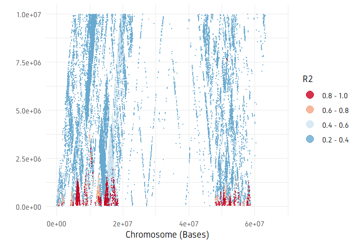
plotPairwiseLD(ld, minr2=0.2, ylim=c(0, 10^7))
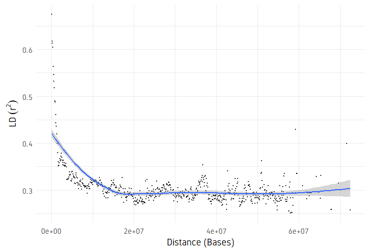
plotDecayLD(ld, minr2=0.25)
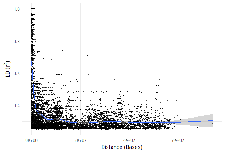
plotDecayLD(ld, minr2=0.25, avgwin=100000)


Comments